040 Working with Pandas#
COM6018
Copyright © 2023–2025 Jon Barker, University of Sheffield. All rights reserved.
In this lab we are going to be working with Pandas. We will see how it can greatly simplify tasks that were quite challenging when using pure Python. To make this clear we will be starting by repeating the analysis we performed in Lab Class 020, ie. producing a plot of the combined Global Warming Potential of atmospheric methane and carbon dioxide over the last three decades.
Start by briefly reviewing the solution notebook for Lab Class 020. Also make sure you have read through the Pandas tutorial notebook that will introduce a lot of the functionality that we will be using in this lab.
Step 1 - Reading in the C02 data#
Before we can use the Pandas package, we will need to import it. Pandas is conventionally imported with the name ‘pd’. Run the cell below which will import both Pandas and NumPy.
import numpy as np
import pandas as pd
First, we will use the pd.read_csv method to load the carbon dioxide data from the CSV file, data/co2.csv. The loaded data will be stored in a Pandas dataframe which we will call co2_df. The CSV file has six fields which we will name as follows: ‘Yr’, ‘Mn’, ‘Dy’, ‘CO2’, ‘NB’, ‘scale’. The co2.csv file has comment lines starting with a ‘%’ symbol. These can be automatically skipped. If you are unsure how to do this then look again at the tutorial notebook, or check the documentation for pd.read_csv.
Complete the cell below such that the TEST cell passes correctly.
co2_df = pd.read_csv('data/co2.csv', comment='%', names=['Yr','Mn','Dy','CO2','NB','scale', 'sta'], skipinitialspace=False)
print(co2_df.dtypes)
Yr         int64
Mn         int64
Dy         int64
CO2       object
NB        object
scale    float64
sta       object
dtype: object
# SOLUTION
co2_df = pd.read_csv('data/co2.csv', comment='%', names=['Yr','Mn','Dy','CO2','NB','scale', 'sta'], skipinitialspace=True)
print(co2_df.dtypes)
Yr         int64
Mn         int64
Dy         int64
CO2      float64
NB       float64
scale    float64
sta       object
dtype: object
# TEST
assert dict(co2_df.iloc[1000]) == {'Yr': np.int64(1960), 'Mn': np.int64(9), 'Dy': np.int64(27), 'CO2': np.float64(313.31), 'NB': np.float64(3.0), 'scale': np.float64(12.0), 'sta': 'mlo'}
print("All tests passed!")
All tests passed!
Note that all the fields have correctly been recognised as numeric types. The year, month and day fields would be more sensibly stored as integers but we are not going to worry about that for now. Note also that reading the data and converting to numeric types has taken one line of code. Compare this to the solution in Lab Class 020 which required quite a lot of code even when using the csv module.
Step 2 - Reading in the CH4 data#
We will now read the methane data (i.e., CH4) from the file data/ch4.csv into a variable which we will call ch4_df. This can be done in a similar way but you will need to modify the read_csv parameters to match the CSV file contents.
Note, the data/ch4.csv file has a row that stores the field names so you will not need to use the names parameter. Note also that the file uses the value ‘-999.99’ to mean that there is a missing reading. You will need to set the ‘na_values’ parameter in order to handle this correctly. If in doubt, check the Pandas read_csv documentation.
Write the code below and then check it by running the test cell.
# SOLUTION
ch4_df = pd.read_csv('data/ch4.csv', comment='#', sep=' ', skipinitialspace=True, na_values='-999.99')
# TEST
assert dict(ch4_df.iloc[1000]) == {'site_code': 'MLO', 'year': np.int64(1989), 'month': np.int64(9), 'day': np.int64(27), 'hour': np.int64(0), 'minute': np.int64(0), 'second': np.int64(0), 'datetime': '1989-09-27T00:00:00Z', 'time_decimal': np.float64(1989.7369863013696), 'midpoint_time': np.int64(622900800), 'value': np.float64(1696.02), 'value_std_dev': np.float64(7.04), 'nvalue': np.int64(7), 'latitude': np.float64(19.536), 'longitude': np.float64(-155.576), 'altitude': np.float64(3437.0), 'elevation': np.float64(3397.0), 'intake_height': np.float64(40.0), 'qcflag': '...'}
Step 3 - Simplifying the data#
We are now going to remove the fields that from each data frame that we are not interested in and rename the others. In our transformed dataframes we want just four columns: year, month, day and co2_concentration for the carbon dioxide data, and year, month, day and ch4_concentration for the methane data.
Making a new dataframe from a subset of columns of an existing one is a very common operation. Check the tutorial notes if you cannot remember how to do this. To rename the fields we can use the DataFrame rename method. These two steps can be written in a single line of code. (Again, compare this with the equivalent step when we implemented this in Lab Class 020 without using Pandas.)
# SOLUTION
co2_df = co2_df.rename(columns={'Yr':'year', 'Mn':'month', 'Dy':'day', 'CO2': 'co2_concentration'})[['year', 'month', 'day', 'co2_concentration']]
ch4_df = ch4_df.rename(columns={'value':'ch4_concentration'})[['year','month','day','ch4_concentration']]
print(ch4_df)
       year  month  day  ch4_concentration
0      1987      1    1                NaN
1      1987      1    2                NaN
2      1987      1    3                NaN
3      1987      1    4                NaN
4      1987      1    5                NaN
...     ...    ...  ...                ...
13630  2024      4   26            1977.78
13631  2024      4   27            1969.78
13632  2024      4   28            1955.87
13633  2024      4   29            1924.00
13634  2024      4   30            1924.86

[13635 rows x 4 columns]
# TEST

assert dict(co2_df.iloc[1000]) == {'year': np.float64(1960.0), 'month': np.float64(9.0), 'day': np.float64(27.0), 'co2_concentration': np.float64(313.31)}
assert dict(ch4_df.iloc[1000]) == {'year': np.float64(1989.0), 'month': np.float64(9.0), 'day': np.float64(27.0), 'ch4_concentration': np.float64(1696.02)}
print('All tests passed!')
All tests passed!
Step 4 - Dealing with missing values#
In the next step we will remove any rows from the dataframes that contain missing concentration values. Check the notes on selecting rows. Hint: you can use the isna() method which returns True for data entries that have NaN values, or, better, you can use the special purpose dropna() method.
# SOLUTION
co2_df = co2_df[~co2_df.co2_concentration.isna()]
ch4_df = ch4_df[~ch4_df.ch4_concentration.isna()]
The same result can be achieved more simply by using the dropna method which removes rows that contain NaN values. Below, the subset parameter is used so that the frames are only dropped in the NaN values are in the co2_concentration or ch4_concentration columns.
# SOLUTION
co2_df = co2_df.dropna(subset=['co2_concentration'])
ch4_df = ch4_df.dropna(subset=['ch4_concentration'])
# TEST
assert len(co2_df) == 18056
assert len(ch4_df) == 12728
print('All tests passed!')
All tests passed!
Step 5 - Fixing the units#
If you remember from Lab 2, the methane concentrations are stored as parts per billion, whereas the carbon dioxide is in parts per million. It will be more convenient to have them both in the same units (i.e., parts per million, ppm). This can be done simply by dividing the ch4_concentration values by 1000.
Scaling a single column of a dataframe is very easy and can be done with a single line. Do this in the cell below.
# SOLUTION
ch4_df.ch4_concentration = ch4_df['ch4_concentration'] / 1000
# TEST
print(ch4_df.ch4_concentration[92])
print('All tests passed!')
1.70002
All tests passed!
Step 6 - Joining the data#
We will now merge our dataframes into a single dataframe using the merge method.
We want to ignore any rows for which there is not both a CO2 and a CH4 measurement, i.e., if for a given day either the CO2 or CH4 measurement is missing then that day will not appear in the merged dataframe. This is called an ‘inner’ join. We can specify that we want an ‘inner’ join by setting the how parameter to inner when we call the merge method.
When performing a merge we need a unique identifier for each row. In our case we will use the combination of the ‘year’, ‘month’ and ‘day’ fields. This is specified using the on parameter.
The merge method returns a new dataframe which we will store in a variable called df.
This step can be completed with a single line. Check the notes if you are unsure.
ch4_df.dtypes, co2_df.dtypes
(year                   int64
 month                  int64
 day                    int64
 ch4_concentration    float64
 dtype: object,
 year                   int64
 month                  int64
 day                    int64
 co2_concentration    float64
 dtype: object)
# SOLUTION
df = co2_df.merge(ch4_df, how='inner', on=['day', 'month', 'year'])
# TEST
assert df['co2_concentration'][0] == 350.84
assert df['ch4_concentration'][0] == 1.70002
print('All tests passed')
All tests passed
Another advantage of using Pandas is that it is very fast. In the cell below, ‘%timeit’ is used to time the merge command. On my machine is takes about 2 ms. This is faster than the function that we wrote in lab 2 when implementing the merge using Python.
%timeit co2_df.merge(ch4_df, how='inner', on=['day', 'month', 'year'])
3.3 ms ± 58.3 μs per loop (mean ± std. dev. of 7 runs, 100 loops each)
Step 7 - Processing the data#
We will continue to follow the steps from Lab 020. We will now combine the CO2 and CH4 concentrations into a single value to represent the total ‘Global Warming Potential’ (GWP) of the gases. Remember, we can do this by converting all gas concentrations into ‘CO2 equivalent’ (CO2e) and then summing them. For CH4 we need to multiple by 28 to compute it’s CO2 equivalent.
So we will make a new column in the dataframe that we will call co2e and which will be equal to co2_concentration + 28 * ch4_concentration. This should be a single line of code. Refer to the notes if you are unsure how to do it. Write this in the cell below.
# SOLUTION
df['co2e'] = df['co2_concentration'] + 28 * df['ch4_concentration']
# TEST
assert df.co2e[0] == 398.44056
print('All tests passed!')
All tests passed!
Step 8 – Plotting the data#
Step 8.1 – Plotting CO2e concentration over time#
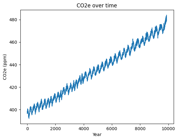
We are now ready to plot the data. We want to see a graph of the CO2e concentration over time.
Previously, in Lab 2, we used the matplotlib library to make the plot. Pandas makes things a bit easier as it has its own plotting tools builtin. The Data Series class has a plot method. e.g. to plot the co2e data we can use df['co2e'].plot() or, equivalently, df.co2e.plot(). The plot method has many parameters that can be used to control the appearance of the plot.
Make a plot with the title ‘CO2e over time’ and with the y-axis labeled as ‘CO2e (ppm)’ and the x-axis labeled as ‘Year’
You will find that the x-axis will be the index of the row, ie from 0 to 9375. We would like it to be the year. Don’t worry about this for now, we will fix it in the next step.
# SOLUTION

my_plot = df['co2e'].plot(title='CO2e over time', ylabel='CO2e (ppm)', xlabel='Year')

Step 8.2 – Plotting by decimal year#
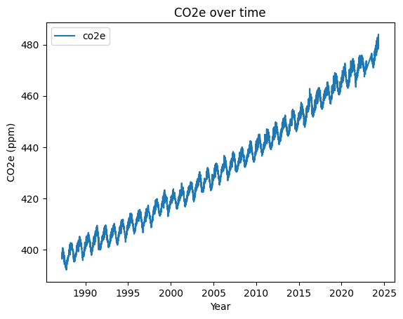
In order to get the x-axis right, we need to turn the date into a decimal number that we can plot against.
Following what we did in Lab 2, we will use the following equation to convert the year, month and day into a single decimial year value,
decimal_year = year + (month - 1) / 12 + (day - 1) / 365
(Note, this equation is not quite correct as it assumes that each month is the same length, but it is good enough for our purposes.)
Add a new column to the DataFrame called decimal_year that is formed using the above equation.
# SOLUTION
df['decimal_year'] = df.year + (df.month - 1) / 12 + (df.day - 1) / 365
# TEST
assert df.decimal_year[0] == 1987.2554794520547
print('All tests passed!')
All tests passed!
We can now plot the co2_e values against decimal year. To plot one column against another we can use the plot method of the dataframe itself and use the ‘x’ and ‘y’ parameters: this looks like df.plot(x='decimial_year, y='co2e')
Try this below, but remember to also give the plot a title and axes labels.
# SOLUTION

my_plot = df.plot(x='decimal_year', y='co2e', title='CO2e over time', ylabel='CO2e (ppm)', xlabel='Year')

We have now used Pandas to repeat everything we did in Lab class 020. Although it has taken a similar number of steps, each step could be completed with a single line of code using pre-existing Pandas functions. Each step will also have run faster.
Step 9 - Extending the analysis#
In this last step we are going to practice what we have just done by adding in data for two more global warming gases: nitrous oxide (N2O) and sulphur hexaflouride (SF6). The data for these gases is stored in the file data/n2o.csv and data/sf6.csv.
Using the techniques from above, read these files and add two new columns to the dataframe, i.e. n2o_concentration and sf6_concentration storing concentrations in parts per million (ppm).
Be careful to interpret the data correctly, i.e. the nitrous oxide data is recorded in parts per billion and the sulfur hexaflouride is measured as parts per trillion (i.e., 10^9). When computing the CO2e figure you can use the following multipliers: 265 for nitrous oxide and 23,500 for sulphur hexaflouride. (These values have been taken from the (IPCC fifth assessment report)[https://ghgprotocol.org/sites/default/files/ghgp/Global-Warming-Potential-Values (Feb 16 2016)_1.pdf])
# SOLUTION

# Load and process n2o data
n2o_df = pd.read_csv('data/n2o.csv', comment='#', sep=' ', skipinitialspace=True)
n2o_df = n2o_df.rename(columns={'N2OcatsMLOyr':'year', 'N2OcatsMLOmon': 'month', 'N2OcatsMLOday':'day', 'N2OcatsMLOm':'n2o_concentration'})[['year','month','day','n2o_concentration']]
n2o_df = n2o_df[~n2o_df.n2o_concentration.isna()]
n2o_df.n2o_concentration = n2o_df['n2o_concentration'] / 1000

# Load and process sf6 data
sf6_df = pd.read_csv('data/sf6.csv', comment='#', sep=' ', skipinitialspace=True)
sf6_df = sf6_df.rename(columns={'SF6catsMLOyr':'year', 'SF6catsMLOmon': 'month', 'SF6catsMLOday':'day', 'SF6catsMLOm':'sf6_concentration'})[['year','month','day','sf6_concentration']]
sf6_df = sf6_df[~sf6_df.sf6_concentration.isna()]
sf6_df.sf6_concentration = sf6_df['sf6_concentration'] / 1000000

# Merge into the main dataframe
df = df.merge(n2o_df, how='inner', on=['day', 'month', 'year'])
df = df.merge(sf6_df, how='inner', on=['day', 'month', 'year'])

# Compute the CO2e figure
df['co2e'] = df['co2_concentration'] + 28 * df['ch4_concentration'] + 265 * df['n2o_concentration'] + 23500 * df['sf6_concentration']
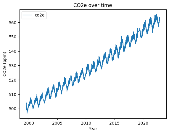
Now make a plot of the total CO2e.
# SOLUTION

my_plot = df.plot(x='decimal_year', y='co2e', title='CO2e over time', ylabel='CO2e (ppm)', xlabel='Year')

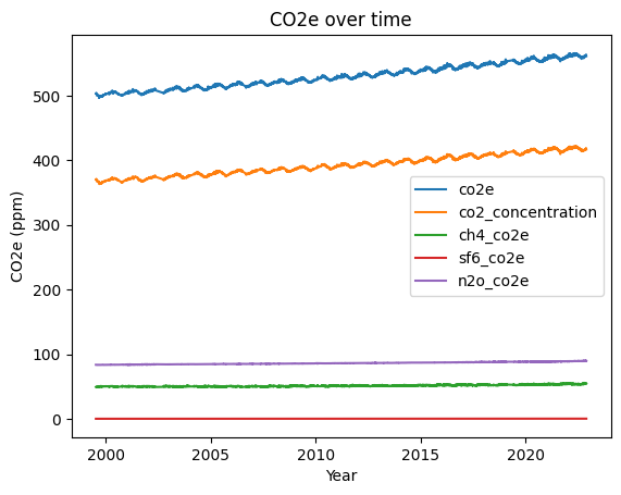
You can plot multiple series on the same axes by setting the plot method’s y parameter to be a list of the names of the series you want to plot, e.g., y=['co2e', 'co2_concentration']. Make a plot that shows the CO2e value for each of the four gases and the total CO2e, all plotted on the same axes. (Hint: in order to do this, you will first need to add new columns to the dataframe to store the CO2e of each of the separate gases.)
Write your code in the cell below.
# SOLUTION
df['ch4_co2e'] = df.ch4_concentration * 28
df['sf6_co2e'] = df.sf6_concentration * 23500
df['n2o_co2e'] = df.n2o_concentration * 265
my_plot = df.plot(x='decimal_year', y=['co2e', 'co2_concentration', 'ch4_co2e', 'sf6_co2e', 'n2o_co2e'], title='CO2e over time', ylabel='CO2e (ppm)', xlabel='Year')

You should see from the plot that although the total CO2e has been steadily rising, nearly all of the increase is due to co2. i.e., the total CO2e line runs in parallel to the CO2 line.
If all have gone well you should have produced a plot looking like the one below.
Conclusion#
In this lab, we learned how to use Pandas to load and process data from CSV files. We also learned how to merge data from multiple sources into a single dataframe, how to construct new DataSeries from existing ones, and how to plot the data using matplotlib.
All of these steps could have been done without Pandas, indeed, we did most of this in Lab 020 just using Python and standard library module. However, using Pandas has made the process considerably simpler to develop and faster to execute. Pandas also contains a lot of more sophisticated functionality that we have not covered here, but which is easy to learn (or look up!) once you have understood the basics.
Copyright © 2023, 2024 Jon Barker, University of Sheffield. All rights reserved.
Copyright © 2023–2025 Jon Barker, University of Sheffield. All rights reserved.


