040 Processing Data with Pandas#
COM6018
Copyright © 2023–2025 Jon Barker, University of Sheffield. All rights reserved.
1. Introduction#
1.1 What is Pandas?#
Up to this point, we have seen that Python’s built-in lists and dictionaries give us a lot of flexibility in how we process data, but this approach is slow and quickly becomes impractical when working with large datasets. NumPy provides a much more efficient alternative for handling numerical data, offering powerful tools for mathematical operations, linear algebra, and the kinds of matrix and vector computations that are common in machine learning. However, NumPy is less effective when we need to deal with more complex, structured data that might include a mix of numbers, text, categories, or missing values. This is where Pandas becomes useful.
Pandas is a third-party, open-source library that was created to meet the needs of data scientists. It builds on the speed of NumPy but adds a wide range of features for handling structured, table-like data, making it possible to work efficiently with datasets that resemble spreadsheets or database tables. While Pandas originally relied on NumPy as its foundation, NumPy was never designed with these kinds of tasks in mind, which led to some inefficiencies. To address this, the recent release of Pandas 2.0 introduced the option of replacing the NumPy backend with Apache Arrow, a framework developed specifically for the fast and efficient processing of large, table-based datasets.
This tutorial is based on Pandas 2.3. The complete documentation can be found at https://pandas.pydata.org/docs/.
1.2 Installing Pandas#
As Pandas is not part of the Python standard library, it must be installed before it can be used. This can be done easily using the pip package manager, or the uv environment manager that we are using with this module.
If Pandas is not installed in your virtual environment, you can install it by typing the following command in your terminal.
uv add pandas
/opt/hostedtoolcache/Python/3.11.14/x64/bin/python: No module named uv
Note: you may need to restart the kernel to use updated packages.
This will install the latest version of Pandas.
To use Pandas in your Python code, you simply need to import it at the start of your program, e.g.,
import pandas as pd
Conventional Python practice is to import Pandas using the alias pd. This is not essential, but it is recommended. Following existing conventions will make your code easier to read for other Python programmers.
1.3 Basic Pandas Concepts#
Pandas is designed for processing structured data much like the data that would be stored in a spreadsheet or a CSV file. Pandas organises data using two basic data structures: the Series and the DataFrame. A Series is a one-dimensional array of data that can be thought of as a single column in a spreadsheet. A DataFrame represents a table of data, which is represented as a collection of Series objects. A DataFrame can be thought of as being similar to an entire spreadsheet. Behind the scenes, Pandas stores this data in NumPy arrays by default, although, as we will see later, it can also be configured to use Apache Arrow.
Pandas has its own type system for representing data. This is largely the same as NumPy’s but extends it to handle additional types such as dates and intervals. Each Series (i.e., each column in a spreadsheet) has its own type, and different Series within the same DataFrame can use different types.
Beyond data storage, Pandas provides powerful tools for processing data. It supports operations such as filtering, joining, and grouping, as well as convenient methods for reading and writing data in many formats, including CSV, Excel, JSON, and SQL. Pandas also includes some basic data visualisation features, which are generally easier to use than the equivalent functionality in Matplotlib.
n the remainder of this tutorial, we will build on these basic concepts step by step. In Section 2, we will look at how to read data from common file formats such as CSV and JSON. Section 3 introduces the DataFrame object in more detail and shows how to select, filter, and inspect data. In Section 4, we will see how to compute summary statistics and group data using the split–apply–combine approach. Section 5 explains how to deal with missing data, while Section 6 demonstrates how to merge and join data from multiple sources.
Sections 7 and 8 cover more advanced topics that are not core to this module but are included for completeness. Section 7 introduces the new Apache Arrow backend, which provides faster and more memory-efficient data handling for large datasets. Section 8 shows how to read data from SQL databases — while we will not be working with SQL in this module, it is useful to know that Pandas can easily read data from database tables.
2. Reading Data#
Pandas has a range of methods for reading data from different standard data formats. For example, it can read Excel spreadsheets directly with a simple read_excel() method. However, continuing from our previous tutorials, we will focus on the commonly used CSV and JSON formats.
2.1 Reading CSV Data#
Reading a CSV file with Pandas can be done with a single line of code:
import pandas as pd
df = pd.read_csv('data/040/windfarm.csv')
The read_csv method will parse the file and return the results as a Pandas DataFrame object. (It is common to use the variable name df for a DataFrame object in simple code examples. You may want to give the DataFrame a more descriptive name when writing more complex code.)
We can now print the resulting DataFrame object to see what it contains:
print(df)
       id   "turbines"   "height"   "power"
0  WF1355           13         53   19500.0
1  WF1364            3         60    8250.0
2  WF1356           12         60   24000.0
3  WF1357           36         60   72000.0
This will produce output that looks like the following,
       id   "turbines"   "height"   "power"
0  WF1355           13         53     19500.0
1  WF1364            3         60      8250.0
2  WF1356           12         60     24000.0
3  WF1357           36         60     72000.0
Note that the read_csv method has read the names of the fields from the first line of the CSV file and used these to name the DataFrame columns. It has placed the names in quotes because quotes were present in the CSV file.
If our CSV file did not have column names in the first line, then we would need to specify them using the names parameter, e.g.,
df = pd.read_csv('data/040/windfarm.no_names.csv', names=['id', 'turbines', 'height', 'power'])
print(df)
       id  turbines  height    power
0  WF1355        13      53  19500.0
1  WF1364         3      60   8250.0
2  WF1356        12      60  24000.0
3  WF1357        36      60  72000.0
Note also how Pandas has added an extra column without a name to the left of the data. This is known as the index column. The index column is used to uniquely identify each row in the DataFrame. Pandas has generated this index for us by giving the rows consecutive integer index values starting from 0. If we want to use a different column as the index, then we can specify this using the index_col parameter, e.g.,
df_id = pd.read_csv('data/040/windfarm.csv', index_col='id')
print(df_id)
        "turbines"  "height"  "power"
id
WF1355          13        53  19500.0
WF1364           3        60   8250.0
WF1356          12        60  24000.0
WF1357          36        60  72000.0
This will produce output looking like the following,
         "turbines"   "height"   "power"
id
WF1355           13         53   19500.0
WF1364            3         60    8250.0
WF1356           12         60   24000.0
WF1357           36         60   72000.0
Tip
You typically want the values in the index column to be unique. If they are not unique, then Pandas will still allow you to use the column as the index, but it will not be able to use some of the more advanced functionality that it offers for indexing. If you are not sure about which column to use as the index, then it is often best not to specify one and to just allow Pandas to create its own index column.
2.2 Reading JSON Data#
Reading JSON data is just as easy as reading CSV data. We can read the climate JSON data from our previous tutorial with a single line of code:
import pandas as pd

df = pd.read_json('data/040/climate.json')
We can now print the resulting DataFrame object to see what it contains:
print(df)
      id            city        country  \
0      1       Amsterdam    Netherlands
1      2          Athens         Greece
2      3      Atlanta GA  United States
3      4        Auckland    New Zealand
4      5       Austin TX  United States
..   ...             ...            ...
100  101  Albuquerque NM  United States
101  102      Vermont IL  United States
102  103    Nashville TE  United States
103  104    St. Louis MO  United States
104  105  Minneapolis MN  United States

                                            monthlyAvg
0    [{'high': 7, 'low': 3, 'dryDays': 19, 'snowDay...
1    [{'high': 12, 'low': 7, 'dryDays': 21, 'snowDa...
2    [{'high': 12, 'low': 2, 'dryDays': 18, 'snowDa...
3    [{'high': 23, 'low': 16, 'dryDays': 24, 'snowD...
4    [{'high': 18, 'low': 6, 'dryDays': 15, 'snowDa...
..                                                 ...
100  [{'high': 10, 'low': -4, 'dryDays': 24, 'snowD...
101  [{'high': 3, 'low': -8, 'dryDays': 18, 'snowDa...
102  [{'high': 9, 'low': -1, 'dryDays': 18, 'snowDa...
103  [{'high': 7, 'low': -4, 'dryDays': 16, 'snowDa...
104  [{'high': -3, 'low': -13, 'dryDays': 20, 'snow...

[105 rows x 4 columns]
Note that the monthlyAvg data which was a list of dictionaries in the JSON file now appears in a single column of the DataFrame. This is not a very convenient format for processing the data. We can use a method called apply() to convert this column into a DataFrame with one column per dictionary in the list.
df_monthly = df['monthlyAvg'].apply(pd.Series)
This creates columns 0, 1, … each containing a dict containing the statistics for that month.
Using apply() a second time on one of the columns can expand the dictionaries into separate columns for each statistic.
print(df_monthly[0].apply(pd.Series))
     high   low  dryDays  snowDays  rainfall
0     7.0   3.0     19.0       4.0      68.0
1    12.0   7.0     21.0       1.0      53.0
2    12.0   2.0     18.0       2.0      99.5
3    23.0  16.0     24.0       0.0      25.6
4    18.0   6.0     15.0       1.0      67.8
..    ...   ...      ...       ...       ...
100  10.0  -4.0     24.0       4.0      10.7
101   3.0  -8.0     18.0      11.0      52.1
102   9.0  -1.0     18.0       8.0      84.4
103   7.0  -4.0     16.0      10.0      69.8
104  -3.0 -13.0     20.0      16.0      19.9

[105 rows x 5 columns]
This is a little complicated, but it is typical of the preprocessing steps we might need to take if working with JSON files that have a complex nested structure. Fortunately, most of the data we will be working with will be in CSV format or in a simple JSON format with a flat structure.
3. The DataFrame Object#
We will now look in a bit more detail at the DataFrame object. For this section we will be using a dataset that records the extent of sea ice in the Arctic and Antarctic. This data is available from the National Snow and Ice Data Center. The data are available in CSV format and we have already downloaded it and saved it in the data directory as seaice.csv.
We will read the data and print the DataFrame,
import pandas as pd

df = pd.read_csv('data/040/seaice.csv')
print(df)
       Year   Month   Day       Extent      Missing  \
0      1978      10    26       10.231          0.0
1      1978      10    28       10.420          0.0
2      1978      10    30       10.557          0.0
3      1978      11     1       10.670          0.0
4      1978      11     3       10.777          0.0
...     ...     ...   ...          ...          ...
26349  2019       5    27       10.085          0.0
26350  2019       5    28       10.078          0.0
26351  2019       5    29       10.219          0.0
26352  2019       5    30       10.363          0.0
26353  2019       5    31       10.436          0.0

                                             Source Data hemisphere
0       ['ftp://sidads.colorado.edu/pub/DATASETS/nsid...      north
1       ['ftp://sidads.colorado.edu/pub/DATASETS/nsid...      north
2       ['ftp://sidads.colorado.edu/pub/DATASETS/nsid...      north
3       ['ftp://sidads.colorado.edu/pub/DATASETS/nsid...      north
4       ['ftp://sidads.colorado.edu/pub/DATASETS/nsid...      north
...                                                  ...        ...
26349  ['ftp://sidads.colorado.edu/pub/DATASETS/nsidc...      south
26350  ['ftp://sidads.colorado.edu/pub/DATASETS/nsidc...      south
26351  ['ftp://sidads.colorado.edu/pub/DATASETS/nsidc...      south
26352  ['ftp://sidads.colorado.edu/pub/DATASETS/nsidc...      south
26353  ['ftp://sidads.colorado.edu/pub/DATASETS/nsidc...      south

[26354 rows x 7 columns]
Note that when printing a DataFrame, Pandas will only show the first and last few rows and columns. We can see from the output that the DataFrame has 26,354 rows and measurements that date back to 1978. But we cannot see the full set of columns.
To get a list of all the columns in the DataFrame, we can use the columns attribute,
print(df.columns)
Index(['Year', ' Month', ' Day', '     Extent', '    Missing', ' Source Data',
       'hemisphere'],
      dtype='object')
This will produce output that looks like the following,
Index(['Year', ' Month', ' Day', '     Extent', '    Missing', ' Source Data',
       'hemisphere'],
      dtype='object')
We can now see that the data are composed of seven columns: year, month, day, extent, missing, source data, and hemisphere. The extent and missing columns record the extent of the sea ice and the number of missing measurements for each day. The source data column records the source of the data. The hemisphere column records whether the data are for the Arctic or Antarctic.
Note that space characters have become incorporated into the column names. This is because the columns in the CSV file had spaces after the commas. We can easily skip these spaces by adding the skipinitialspace=True parameter to the read_csv() method,
import pandas as pd

df = pd.read_csv('data/040/seaice.csv', sep=',', skipinitialspace=True)
print(df.columns)
Index(['Year', 'Month', 'Day', 'Extent', 'Missing', 'Source Data',
       'hemisphere'],
      dtype='object')
3.1 Selecting a Column#
We can select a single column from the DataFrame using the column name as an index.
extent = df['Extent']
print(extent)
0        10.231
1        10.420
2        10.557
3        10.670
4        10.777
          ...
26349    10.085
26350    10.078
26351    10.219
26352    10.363
26353    10.436
Name: Extent, Length: 26354, dtype: float64
This will produce output looking like the following,
0        10.231
1        10.420
2        10.557
3        10.670
4        10.777
          ...
26349    10.085
26350    10.078
26351    10.219
26352    10.363
26353    10.436
Name: Extent, Length: 26354, dtype: float64
Notice how this looks a bit different from when we printed the DataFrame. This is because the column is not a DataFrame; it is a Series. Remember, Pandas uses the Series object for storing individual columns of data. We can check this by printing the type of the column,
print(type(df))  # This will print <class 'pandas.core.frame.DataFrame'>
extent = df['Extent']
print(type(extent))  # This will print <class 'pandas.core.series.Series'>
<class 'pandas.core.frame.DataFrame'>
<class 'pandas.core.series.Series'>
The Series object has a specific type (called its dtype). In this case the type is float64 which means that the data are stored as 64-bit floating point numbers. We can check the type of the data in a Series using the dtype attribute. Or, more conveniently, we can retrieve the data type of all the columns in the DataFrame using the DataFrame’s dtypes attribute. Let’s do that now,
print(df.dtypes)
Year             int64
Month            int64
Day              int64
Extent         float64
Missing        float64
Source Data     object
hemisphere      object
dtype: object
This will produce output looking like the following,
Year             int64
Month            int64
Day              int64
Extent         float64
Missing        float64
Source Data     object
hemisphere      object
dtype: object
We can see that the Year, Month and Day have integer values; the Extent and Missing columns have floating-point values; and the Source Data and hemisphere columns have ‘object’ values.
Pandas has inferred these types from the content of the CSV file. It usually guesses correctly, but it can sometimes get it wrong. If it is unsure it will typically default to the ‘object’ type. This has happened for the ‘Source Data’ and ‘hemisphere’ columns which should be strings. We can fix this by explicitly converting these columns to strings using the astype() method,
df['Source Data'] = df['Source Data'].astype("string")
df['hemisphere'] = df['hemisphere'].astype("string")
print(df.dtypes)
Year                    int64
Month                   int64
Day                     int64
Extent                float64
Missing               float64
Source Data    string[python]
hemisphere     string[python]
dtype: object
A Series object is much like a list, and we can use indexes and slicing operators to reference elements in the Series. For example, we can get the first element in the Series using,
extent = df['Extent']
print(extent[0])  # print the first element
10.231
or we can retrieve the sequence of elements from the 6th to 10th with,
extent = df['Extent']
print(extent[5:10]) # print a sub-Series from index 5 to 9
5    10.968
6    11.080
7    11.189
8    11.314
9    11.460
Name: Extent, dtype: float64
(Recall that the first element of a Series has index 0, so the 10th element has index 9. The slice notation a:b means to go from index a to b-1 inclusive.)
3.2 Selecting a Row#
We can select a single row from the DataFrame using the iloc attribute. This attribute takes a single integer index and returns a Series containing the data from the row at that index. For example, to select the first row, we can use,
row = df.iloc[0]
print(row)
Year                                                        1978
Month                                                         10
Day                                                           26
Extent                                                    10.231
Missing                                                      0.0
Source Data    ['ftp://sidads.colorado.edu/pub/DATASETS/nsidc...
hemisphere                                                 north
Name: 0, dtype: object
Notice how the results have been returned as a Series object. We can check this by printing the type of the row,
print(type(row)) # This will print <class 'pandas.core.series.Series'>
<class 'pandas.core.series.Series'>
DataFrames are a collection of Series objects representing the columns, However, if we extract a single row, this will also be returned as a Series object, i.e., representing the values in that row. The dtype of the row series is ‘object’. An ‘object’ type can basically store anything, so it is being used here because each element in the row Series has a different type.
Alternatively, we can extract a range of rows using slicing,
rows = df.iloc[0:5]
print(rows)
   Year  Month  Day  Extent  Missing  \
0  1978     10   26  10.231      0.0
1  1978     10   28  10.420      0.0
2  1978     10   30  10.557      0.0
3  1978     11    1  10.670      0.0
4  1978     11    3  10.777      0.0

                                         Source Data hemisphere
0  ['ftp://sidads.colorado.edu/pub/DATASETS/nsidc...      north
1  ['ftp://sidads.colorado.edu/pub/DATASETS/nsidc...      north
2  ['ftp://sidads.colorado.edu/pub/DATASETS/nsidc...      north
3  ['ftp://sidads.colorado.edu/pub/DATASETS/nsidc...      north
4  ['ftp://sidads.colorado.edu/pub/DATASETS/nsidc...      north
Note that a collection of rows is still a DataFrame. We can check this by printing the type of the variable rows,
print(type(rows))
<class 'pandas.core.frame.DataFrame'>
Basically, if we have a single row or column, then we are dealing with a Series, but if we have multiple rows and columns, then we are dealing with a DataFrame.
3.3 Filtering a DataFrame#
Very often in data science, we need to select some subset of our data based on some condition, e.g., all cities where the population is greater than 1 million or all years where the average temperature was less than 15 degrees Celsius. Or, more simply, we may wish to select every row that has an even index value. Alternatively, we may want to remove various columns from the DataFrame, i.e., those representing fields that we are not interested in. We will refer to these operations that take a DataFrame and return another smaller DataFrame as filtering operations. In this section, we will look at a few simple examples.
3.3.1 Removing or Selecting Columns#
After loading our data, we may want to remove columns that we are not interested in. This is easily done using the drop() method. For example, to make it easier to print the data frame, we will remove the Source Data column using,
df = df.drop(columns=['Source Data'])
There are now only 6 columns in the DataFrame and they can all be viewed at once,
print(df)
       Year  Month  Day  Extent  Missing hemisphere
0      1978     10   26  10.231      0.0      north
1      1978     10   28  10.420      0.0      north
2      1978     10   30  10.557      0.0      north
3      1978     11    1  10.670      0.0      north
4      1978     11    3  10.777      0.0      north
...     ...    ...  ...     ...      ...        ...
26349  2019      5   27  10.085      0.0      south
26350  2019      5   28  10.078      0.0      south
26351  2019      5   29  10.219      0.0      south
26352  2019      5   30  10.363      0.0      south
26353  2019      5   31  10.436      0.0      south

[26354 rows x 6 columns]
Rather than removing columns, an alternative is to actively select the subset of columns that we wish to keep. This is done with the following indexing notation,
df = df[['Year', 'Month', 'Day', 'Extent', 'Missing', 'hemisphere']]
3.3.2 Selecting Rows#
Very often when analysing data we want to select a subset of the samples that match some criterion, i.e., to select a subset of the rows in our DataFrame. This is very straightforward in Pandas and is done using a Boolean expression as the index value.
For example, let’s say we want to select all the rows where the sea ice extent value is less than 5.0. We can do this using,
selector = df['Extent'] < 5.0
df_low_extent = df[selector]
We have done this in two steps. The first line takes the Extent Series and compares every value to 5.0. This produces a Series of boolean (i.e., True or False) values which we have stored in a variable called selector. The second line uses this boolean Series as an index which has the effect of selecting only the rows for which the value is True.
If we now print the resulting DataFrame we can see that it only contains about 3000 rows of the original 26,354 rows in the dataset; i.e., these are the samples where the sea ice extent has fallen below 5.0 billion square kilometres.
print(df_low_extent)
       Year  Month  Day  Extent  Missing hemisphere
8874   2007      8   20   4.997      0.0      north
8875   2007      8   21   4.923      0.0      north
8876   2007      8   22   4.901      0.0      north
8877   2007      8   23   4.872      0.0      north
8878   2007      8   24   4.837      0.0      north
...     ...    ...  ...     ...      ...        ...
26296  2019      4    4   4.564      0.0      south
26297  2019      4    5   4.730      0.0      south
26298  2019      4    6   4.856      0.0      south
26299  2019      4    7   4.902      0.0      south
26300  2019      4    8   4.993      0.0      south

[2988 rows x 6 columns]
They are ordered by year. What do you notice about the earliest year of these data? Recall that the original complete dataset had recordings going back to 1978, but all the monthly recordings where the extent of the sea ice fallen below 5.0 billion square kilometres have occurred since 2007. Is this something that might have happened by chance, or is it evidence of a trend in the data? We will see how to answer such questions a little later in the module.
Let us say that we now just want to look at the Arctic data. We can do this by selecting only the rows where the hemisphere is ‘north’. We can do this using the eq() method,
filter = df['hemisphere'].eq('north')
If we wanted to combine these two filters to select only the rows where the sea ice extent is less than 5.0 billion square kilometres and the hemisphere is ‘north’, we could do this using the & operator,
filter = (df['hemisphere'].eq('north')) & (df['Extent'] < 5.0)
df_low_extent_north = df[filter]
Caution
When combining multiple filter expression use the operators & (and), | (or) and ~ (not) rather than the keywords and, or and not. The latter keywords will not work for combining filter expressions.
print(df_low_extent_north)
       Year  Month  Day  Extent  Missing hemisphere
8874   2007      8   20   4.997      0.0      north
8875   2007      8   21   4.923      0.0      north
8876   2007      8   22   4.901      0.0      north
8877   2007      8   23   4.872      0.0      north
8878   2007      8   24   4.837      0.0      north
...     ...    ...  ...     ...      ...        ...
12932  2018      9   29   4.846      0.0      north
12933  2018      9   30   4.875      0.0      north
12934  2018     10    1   4.947      0.0      north
12935  2018     10    2   4.988      0.0      north
12936  2018     10    3   4.975      0.0      north

[339 rows x 6 columns]
This leaves just 339 rows.
Note
Be careful to use parentheses around each filter expression above. The & operator has a higher precedence than the < operator so if you do not use parentheses then it will still be a valid expression but it will not work in the way you expected.
Note that we use a very similar indexing syntax, i.e., df[selector], for selecting both rows and columns. The difference is that when selecting rows we use a boolean series as the index value, whereas when selecting columns we use a list of column names as the index value. This can be a little confusing at first, but you will soon get used to it.
4. Grouping and averaging values#
Up to this point, we have mainly focused on how to read, inspect, and filter data in Pandas. In practice, however, much of data analysis involves summarising information — for example, finding averages, totals, or other statistics that describe entire columns or subsets of the data. Pandas provides concise and efficient ways to compute such statistics, either across all rows or within meaningful groups (such as by year, category, or location).
In this section, we will first look at simple operations that compute statistics over entire columns, and then explore how to group data so that these statistics can be computed separately for each group.
4.1 Operating on columns#
There are many operations that we might apply over an entire column to compute some ‘statistic’ of that column. For example, we might want to compute a columns minimum, maximum, mean, median, standard deviation, etc. The Series object provides many methods to make this easy.
For example, to compute the mean of the Extent column we can use,
mean_value = df['Extent'].mean()
print(mean_value)
11.494986301889657
We can also calculate the minimum and maximum values in a similar way,
print(df['Extent'].min(), df['Extent'].max())
2.08 20.201
For convenience, the DataFrame object provides a describe() method that will compute and display the basic statistics for all columns in the DataFrame that have numerical values. For example,
print(df.describe())
               Year         Month           Day        Extent       Missing
count  26354.000000  26354.000000  26354.000000  26354.000000  26354.000000
mean    2000.591941      6.507399     15.740685     11.494986      0.000003
std       10.896821      3.451938      8.801607      4.611734      0.000227
min     1978.000000      1.000000      1.000000      2.080000      0.000000
25%     1992.000000      4.000000      8.000000      7.601000      0.000000
50%     2001.000000      7.000000     16.000000     12.217000      0.000000
75%     2010.000000     10.000000     23.000000     15.114000      0.000000
max     2019.000000     12.000000     31.000000     20.201000      0.024000
This will print the following table:
               Year         Month           Day        Extent       Missing
count  26354.000000  26354.000000  26354.000000  26354.000000  26354.000000
mean    2000.591941      6.507399     15.740685     11.494986      0.000003
std       10.896821      3.451938      8.801607      4.611734      0.000227
min     1978.000000      1.000000      1.000000      2.080000      0.000000
25%     1992.000000      4.000000      8.000000      7.601000      0.000000
50%     2001.000000      7.000000     16.000000     12.217000      0.000000
75%     2010.000000     10.000000     23.000000     15.114000      0.000000
max     2019.000000     12.000000     31.000000     20.201000      0.024000
The table shows the number of items (count), mean, standard deviation (std), minimum (min), maximum (max) and the 25th, 50th, and 75th percentiles of the data in each column. Note that the 50th percentile is the same as the median. These statistics will be more meaningful for some columns than for others. For example, in the above the mean and standard deviation of the Month and Day columns are not very meaningful. Nevertheless, the describe() method is very useful for getting a quick overview of the data and is often the first thing we will do when we load a new dataset.
4.2 Grouping data#
n the previous section, we computed statistics across entire columns of the dataset. However, it is often more useful to calculate these statistics separately for meaningful subsets of the data — for example, to find the mean sea-ice extent for each year, each month, or for the northern and southern hemispheres independently. To do this, we need a way to divide the data into groups and then compute statistics within each group.
Pandas provides a simple and consistent pattern for this type of operation, often referred to as the “split–apply–combine” process:
Split (group): divide the DataFrame into groups based on one or more key columns.
Apply (process): perform an operation independently on each group — for example, computing a mean, minimum, or count.
Combine: bring the results of these operations back together into a new DataFrame or Series.
This split–apply–combine pattern is exactly the sequence that Pandas follows when we use the groupby() method. We first tell Pandas how to split the data into groups, then apply one or more operations to each group, and finally combine the results into a new object for inspection or further analysis.
In the combine step, Pandas also creates an index that reflects the grouping keys. When you group by more than one column, the resulting object will use a hierarchical or “MultiIndex,” where each level corresponds to one of the grouping columns.
For example, to group the data by month we can use,
grouped = df.groupby('Month')
This returns a special DataFrameGroupBy object. This object does not immediately compute anything — it simply records how the data have been split into groups. We can then compute statistics on those groups by selecting a column and using the same methods that we used earlier. For example, to compute the mean sea-ice extent for each month we can use,
print(grouped['Extent'].mean())
Month
1      9.587706
2      9.057401
3      9.621926
4     10.678099
5     11.637163
6     12.476158
7     12.563403
8     12.288473
9     12.265863
10    13.044214
11    13.152069
12    11.514823
Name: Extent, dtype: float64
TThe code above produces a mean value for each month of the year (1 is January, 2 is February, etc.). Notice how the amount of ice reaches a maximum in November and a minimum in February. This might seem somewhat surprising — the maximum and minimum are not six months apart, as might be expected. Note, however, that when we grouped by month we included both Northern and Southern Hemisphere measurements, so this mean will be the average across both hemispheres, which can lead to an unintuitive result.
Let us say that we wanted to look at the sea-ice extent for each month but separately for the northern and southern hemispheres. We now want to group by both month and hemisphere. We can do this easily by passing a list of column names to the groupby() method,
grouped = df.groupby(['hemisphere', 'Month'])
print(grouped['Extent'].mean())
hemisphere  Month
north       1        14.176006
            2        15.044512
            3        15.205876
            4        14.481141
            5        13.072172
            6        11.516788
            7         9.090173
            8         6.784248
            9         5.988981
            10        7.929377
            11       10.448120
            12       12.638618
south       1         4.999406
            2         3.070290
            3         4.037976
            4         6.875058
            5        10.202155
            6        13.435529
            7        16.036633
            8        17.792698
            9        18.542745
            10       18.159051
            11       15.856019
            12       10.391028
Name: Extent, dtype: float64
When grouping by multiple fields, the combine step produces a result indexed by both grouping keys. In Pandas, this is represented as a ‘MultiIndex’, where the first level corresponds to the first grouping column (hemisphere) and the second level corresponds to the second grouping column (Month). You can later reset this MultiIndex using reset_index() if you prefer to work with a flat DataFrame.
For example, if we want to convert the grouped means into an ordinary DataFrame with regular columns instead of a hierarchical index, we can do:
grouped = df.groupby(['hemisphere', 'Month'])
monthly_means = grouped['Extent'].mean().reset_index()
print(monthly_means.head())
  hemisphere  Month     Extent
0      north      1  14.176006
1      north      2  15.044512
2      north      3  15.205876
3      north      4  14.481141
4      north      5  13.072172
This produces a DataFrame where hemisphere, Month, and Extent are all standard columns rather than index levels. This makes the data easier to manipulate or save to a file.
We now see that in the Arctic, sea ice extent reaches a maximum monthly average in March and a minimum in September. In the Antarctic, sea ice extent reaches a maximum month average in September and a minimum in February. This is more in line with what we might expect — that is, the maxima and minima are about six months apart. The dates might seem a little later than what you would consider to be the peak of winter and summer. This is because of the way water stores heat: the oceans take a long time to cool down and warm up, so the coldest and warmest months are not necessarily those with the shortest and longest days. You can now also see that the Antarctic sea-ice extent is much more variable than the Arctic sea-ice extent.
Let us now consider how we would examine the Arctic and Antarctic sea-ice minimum over the years. We can do this by grouping by hemisphere and year and then selecting the minimum value in each group,
grouped = df.groupby(['hemisphere', 'Year'])
print(grouped['Extent'].min())
hemisphere  Year
north       1978    10.231
            1979     6.895
            1980     7.533
            1981     6.902
            1982     7.160
                     ...
south       2015     3.544
            2016     2.616
            2017     2.080
            2018     2.150
            2019     2.444
Name: Extent, Length: 84, dtype: float64
(Here again, the result uses a MultiIndex: hemisphere and year.)
Pandas has built-in methods to make plots. Below we are making a plot and then getting the figure from the plot and saving it to a file. The resulting plot is being imported back into these notes.
grouped = df.groupby(['hemisphere', 'Year'])
ice_extent = grouped['Extent'].min()['north']

my_plot = ice_extent.plot()
my_plot.get_figure().savefig("figures/040_1.jpeg")
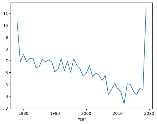
It will generate the following plot.
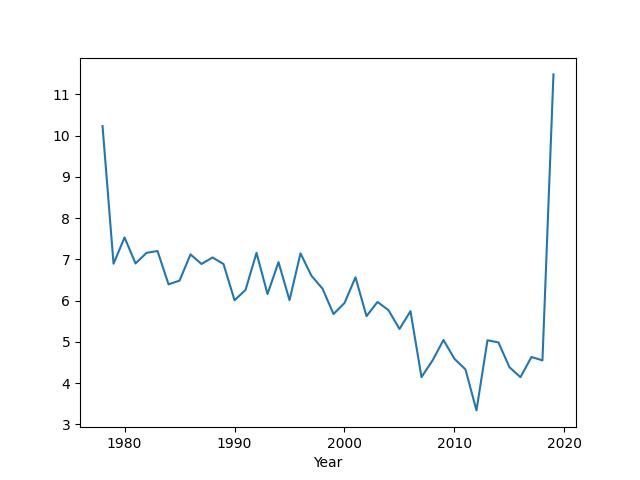
You can see that the sea ice extent has been broadly trending downwards but the values at the extremes of the x-axis look a bit odd, i.e., there are very large values for the first and last year in the dataset. This is an ‘artifact’ caused by the data for these years being incomplete. The data for 1978 only start in November and the data for 2019 only go up to July. The code has computed the minimum for the few months that are available, but this is not representative of the minimum for the full year. We can fix this problem by simply removing these years from the data before plotting.
To remove the first and last values in a Series we can use the familiar slicing notation that we saw when using NumPy, ‘[1:-1]’. So, the code will now look like
grouped = df.groupby(['hemisphere', 'Year'])
ice_extent = grouped['Extent'].min()['north']
ice_extent = ice_extent[1:-1]  # remove first and last years

my_plot = ice_extent.plot(title='Arctic sea ice minimum', ylabel='million square kilometres (million km²)', xlabel='Year')
my_plot.get_figure().savefig("figures/040_2.jpeg")
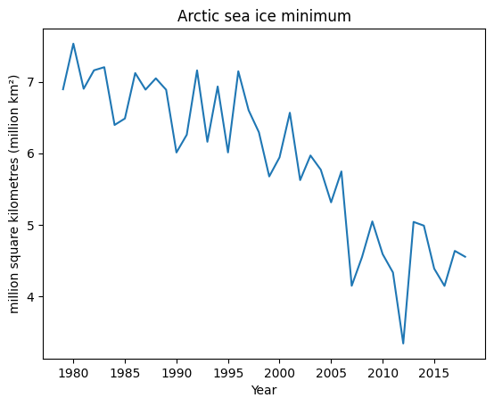
It will generate the following plot.
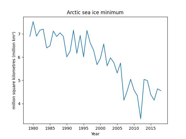
Notice how the sea ice minimum fluctuates seemingly at random from year to year. This kind of unexplained variation in data is often referred to as noise. However, ignoring the fluctuations, we can see that there also appears to be a downward trend in the sea ice minimum. If we want to be sure that there is a genuine downward trend and that the low values in recent years are not just part of the usual random fluctuations, then we need to perform some statistical analysis. We will look at how to do this later in the module.
5. Dealing with Missing Data#
Very often we need to work with datasets that have ‘missing values’, i.e., for one or more fields in the data there is no value available. These are typically encoded in the data file using a special symbol such as ‘NaN’. For example, we may have some employee data that records an ID, a surname and age, and a gender, but there may be some employees that have not provided either their age or gender or both.
We can read and display some example data.
df = pd.read_csv('data/040/employee.csv')
Note, below, the presence of ‘NaN’ in the age and gender columns.
print(df)
   ID    Surname   Age  Gender
0   1      Smith  32.0    Male
1   2    Johnson  45.0  Female
2   3   Gonzalez   NaN     NaN
3   4         Li  37.0  Female
4   5      Brown  41.0    Male
5   6  Rodriguez  29.0  Female
6   7      Kumar  32.0     NaN
7   8      Lopez  36.0  Female
8   9     Nguyen   NaN    Male
9  10      Patel  40.0    Male
There are some methods to test for the presence of these missing values. For example, the isnull() method will produce a new DataFrame of boolean values with a value of True in every location where an item of data is missing.
print(pd.isnull(df))
      ID  Surname    Age  Gender
0  False    False  False   False
1  False    False  False   False
2  False    False   True    True
3  False    False  False   False
4  False    False  False   False
5  False    False  False   False
6  False    False  False    True
7  False    False  False   False
8  False    False   True   False
9  False    False  False   False
Typically if we have missing values we will need to take some action to deal with them before progressing with our analysis. Depending on the situation, the most appropriate action might be to simply remove the rows with missing values, or to fill in the missing values with some sensible default value, or to use some more sophisticated method for estimating what the missing values would have been if they had been present.
5.1 Filling missing data with a fixed value#
Sometimes our data will contain missing values, which Pandas represents as NaN. We can replace these with something more useful or readable using the fillna method. For instance, if we want to display the data and make it clearer, we might choose to replace missing values in the Gender column with the string “Gender not provided”.
This can be done as follows:
df.fillna({"Gender":"Gender not provided"}, inplace=True)
Here, we pass a dictionary to fillna, where the key is the column name (“Gender”) and the value is what we want to use as the replacement. The inplace=True argument means the DataFrame will be updated directly, without creating a new copy.
After the replacement, our DataFrame will be as follows.
print(df)
   ID    Surname   Age               Gender
0   1      Smith  32.0                 Male
1   2    Johnson  45.0               Female
2   3   Gonzalez   NaN  Gender not provided
3   4         Li  37.0               Female
4   5      Brown  41.0                 Male
5   6  Rodriguez  29.0               Female
6   7      Kumar  32.0  Gender not provided
7   8      Lopez  36.0               Female
8   9     Nguyen   NaN                 Male
9  10      Patel  40.0                 Male
The idea of modifying objects in place is common in Pandas, and many methods provide an inplace parameter. For large DataFrames, modifying data in place can reduce memory overhead because it avoids creating a new copy. However, this style of programming can also introduce subtle bugs. For example, if a function both modifies a DataFrame in place and returns it, the caller might not realise that the original DataFrame they passed in has already been altered. This kind of unexpected behaviour can be difficult to track down.
A safer and more transparent approach is to leave inplace=False (the default) and explicitly assign the result of the operation to a new variable. This “copy semantics” style makes it clearer what is happening and is generally recommended unless you are certain that performance or memory usage requires the in-place approach. In fact, the Pandas developers are moving away from the use of inplace altogether, and some methods in recent versions no longer support it.
For example, the same operation can be written using copy semantics like this:
new_df = df.fillna({"Gender":"Gender not provided"})
print(new_df)
   ID    Surname   Age               Gender
0   1      Smith  32.0                 Male
1   2    Johnson  45.0               Female
2   3   Gonzalez   NaN  Gender not provided
3   4         Li  37.0               Female
4   5      Brown  41.0                 Male
5   6  Rodriguez  29.0               Female
6   7      Kumar  32.0  Gender not provided
7   8      Lopez  36.0               Female
8   9     Nguyen   NaN                 Male
9  10      Patel  40.0                 Male
The fillna method has other useful options such as a method parameter that can fill the missing value with the previous or next valid observation in the Series. This behaviour is useful for sequential data, e.g., data ordered by date, for example. For example, if there is a weather station but it has failed to record a temperature on a particular day, then we might opt to fill in the missing value with the temperature recorded on the previous day as this is likely to be a reasonably good estimate.
5.2 Filling missing values using ‘mean imputation’#
Another common strategy for filling missing values in numeric data is to fill the missing values with the mean of the values that are present. In the data science literature, this is known as ‘mean imputation’. This might be a sensible way of treating our missing employee age data and can be easily done using,
df.fillna({'Age':df['Age'].mean()}, inplace=True)
This will produce the following.
print(df)
   ID    Surname   Age               Gender
0   1      Smith  32.0                 Male
1   2    Johnson  45.0               Female
2   3   Gonzalez  36.5  Gender not provided
3   4         Li  37.0               Female
4   5      Brown  41.0                 Male
5   6  Rodriguez  29.0               Female
6   7      Kumar  32.0  Gender not provided
7   8      Lopez  36.0               Female
8   9     Nguyen  36.5                 Male
9  10      Patel  40.0                 Male
Note how the missing age values for Gonzalez and Nguyen have now been replaced with 36.5. Obviously, this is unlikely to be their true ages, but it might be a sensible guess to use in the analysis stages that are going to follow.
Treatment of missing data is a big topic and something we will return to later in the module.
6. Collating data#
Very often, as Data Scientists, we need to combine data from different sources. For example, we might have two separate datasets that are linked by a shared field, such as the customer ID, date, or location. These will typically start life as separate files. These can be read into two separate DataFrames but in order to understand the data we will generally need to combine these DataFrames into a new common DataFrame, in some way.
In the simple example below, we will consider two different sets of atmospheric gas readings, carbon dioxide and methane that have been measured at the same location over time but are stored separately in the files co2.csv and ch4.csv. (The file names are based on the chemical formulae for carbon dioxide and methane, CO2 and CH4, respectively).
Let us imagine that the first few rows of these tables look like this
year, month, day, co2
2020, 1, 02, 442
2020, 1, 03, 444
2020, 1, 04, 441
2020, 1, 07, 446
and this,
year, month, day, ch4
2020, 1, 02, 442
2020, 1, 03, 444
2020, 1, 05, 441
2020, 1, 06, 442
2020, 1, 07, 446
We can see that both tables share the same year, month and day columns but each has its own unique column for the gas concentration measurement. We can also see that the data are not recorded on every day: on some days there is both a carbon dioxide and a methane measurement, on some there is only one or the other and on some dates there is neither. We will now consider different ways in which these datasets can be combined.
6.1 Combining DataFrames using the merge method#
To make the task a bit more instructive, the above data have some missing entries, e.g., entries for days 05 and 06 are missing from the CO2 data. The entry for day 04 is missing from the CH4 data. In a well-designed dataset these might have been recorded with NaN values but often there are just gaps in the data.
We can read these tables using,
co2_df = pd.read_csv('data/040/co2_ex.csv', skipinitialspace=True)
ch4_df = pd.read_csv('data/040/ch4_ex.csv',  skipinitialspace=True)
print(co2_df)
print(ch4_df)
   year  month  day  co2
0  2020      1    2  442
1  2020      1    3  444
2  2020      1    4  441
3  2020      1    7  446
   year  month  day  ch4
0  2020      1    2  442
1  2020      1    3  444
2  2020      1    5  441
3  2020      1    6  442
4  2020      1    7  446
We can now merge the tables. To do this, we need to pick a column to merge on. This is typically a key-like value that uniquely identifies the data entry (i.e., the row) and appears in both tables. If no one column is unique then we can use a collection of columns to merge on. For example, in our data, neither the year, month nor day would be a unique identifier if taken in isolation, but the three together form a unique set of values (i.e., because there is only one measurement per day, no two rows have an identical year, month and day). So we will use on=['year', 'month', 'day'].
We can then merge in four different ways: inner, outer, left or right. These differ in how they treat missing values: inner will only merge rows which exist in both DataFrames (i.e., if you think of this a merging two sets then this would be an ‘intersection’); outer will include rows that exist in either of the two DataFrames (i.e., in terms of sets, this would be a ‘union’); left only includes rows which are in the first DataFrame and right only those in the second. This can be most easily understood by comparing the outputs below.
Merging CO2 and CH4 using an
innermerge:
combined_df = co2_df.merge(ch4_df, on=['year', 'month', 'day'], how='inner')
print(combined_df)
   year  month  day  co2  ch4
0  2020      1    2  442  442
1  2020      1    3  444  444
2  2020      1    7  446  446
Merging CO2 and CH4 using an
outermerge:
combined_df = co2_df.merge(ch4_df, on=['year', 'month', 'day'], how='outer')
print(combined_df)
   year  month  day    co2    ch4
0  2020      1    2  442.0  442.0
1  2020      1    3  444.0  444.0
2  2020      1    4  441.0    NaN
3  2020      1    5    NaN  441.0
4  2020      1    6    NaN  442.0
5  2020      1    7  446.0  446.0
Merging CO2 and CH4 using a
leftmerge:
combined_df = co2_df.merge(ch4_df, on=['year', 'month', 'day'], how='left')
print(combined_df)
   year  month  day  co2    ch4
0  2020      1    2  442  442.0
1  2020      1    3  444  444.0
2  2020      1    4  441    NaN
3  2020      1    7  446  446.0
Merging CO2 and CH4 using a
rightmerge:
combined_df = co2_df.merge(ch4_df, on=['year', 'month', 'day'], how='right')
print(combined_df)
   year  month  day    co2  ch4
0  2020      1    2  442.0  442
1  2020      1    3  444.0  444
2  2020      1    5    NaN  441
3  2020      1    6    NaN  442
4  2020      1    7  446.0  446
In all cases, in the resulting table, any missing values will be automatically filled in with NaNs.
Warning: Typically, the join columns act as a unique key. What happens if we choose columns that are not unique? Below we attempt to join on the ‘year’ column which is actually the same for all our rows, i.e.,
combined_df = co2_df.merge(ch4_df, on=['year'], how='inner')
print(combined_df)
    year  month_x  day_x  co2  month_y  day_y  ch4
0   2020        1      2  442        1      2  442
1   2020        1      2  442        1      3  444
2   2020        1      2  442        1      5  441
3   2020        1      2  442        1      6  442
4   2020        1      2  442        1      7  446
5   2020        1      3  444        1      2  442
6   2020        1      3  444        1      3  444
7   2020        1      3  444        1      5  441
8   2020        1      3  444        1      6  442
9   2020        1      3  444        1      7  446
10  2020        1      4  441        1      2  442
11  2020        1      4  441        1      3  444
12  2020        1      4  441        1      5  441
13  2020        1      4  441        1      6  442
14  2020        1      4  441        1      7  446
15  2020        1      7  446        1      2  442
16  2020        1      7  446        1      3  444
17  2020        1      7  446        1      5  441
18  2020        1      7  446        1      6  442
19  2020        1      7  446        1      7  446
This has taken the set of rows from each table that share the same year and made new rows using every possible pairing of rows in these sets. Also because ‘month’ and ‘day’ were not in the join, the new DataFrame now has separate month and day columns coming from the two original DataFrames which have been automatically distinguished with the suffixes ‘_x’ and ‘_y’. There are cases when we might want this behaviour, but if your output is looking like this, it is more likely that it’s because you have set the on parameter incorrectly.
6.2 Combining DataFrames using the join method#
The join method is very similar to merge except that it uses the DataFrame index to decide which rows to combine. It can be thought of as a special case of merge. However, it is often more convenient and faster to use. If the DataFrame already has a meaningful index, then this is very easy to use; e.g., perhaps a product ID column is being used as the index and we have two DataFrames containing product sales for different product ranges that we wish to join.
In our case, if working with the CO2 and CH4 data from above, in order to use join, we would first need to make an index using the year, month, and day columns. We can do this using the set_index method, like this:
co2_df_indexed = co2_df.set_index(['year', 'month', 'day'])
ch4_df_indexed = ch4_df.set_index(['year', 'month', 'day'])
print(co2_df_indexed)
print(ch4_df_indexed)
                co2
year month day
2020 1     2    442
           3    444
           4    441
           7    446
                ch4
year month day
2020 1     2    442
           3    444
           5    441
           6    442
           7    446
We can now perform the join. Again, as with merge, we can join using inner, outer, left or right.
combined_df = co2_df_indexed.join(ch4_df_indexed, how='outer')
print(combined_df)
                  co2    ch4
year month day
2020 1     2    442.0  442.0
           3    444.0  444.0
           4    441.0    NaN
           5      NaN  441.0
           6      NaN  442.0
           7    446.0  446.0
Comparing merge and join, merge is more versatile because it can merge on any column, whereas join can only merge on the index. So you might wonder why we have a join method at all? The answer is that the join method works internally in a very different way from merge that exploits special properties of the DataFrame index. For large DataFrames, join is generally much faster than merge and so should be preferred if its use is possible.
7. Using the Apache Arrow backend#
Pandas 2.x can store DataFrame columns using Apache Arrow instead of NumPy. Arrow provides efficient, columnar, nullable types (including true nullable integers) and can speed up I/O and many column operations. Some key benefits are:
Faster operations – many columnar operations (e.g., filtering, arithmetic) can be executed more efficiently on Arrow data.
Smaller memory footprint – Arrow uses compact, type-specific encodings and lightweight null bitmaps, reducing memory use for large DataFrames.
True nullable types – integers, booleans, and other types can natively represent missing values without falling back to slower object arrays.
Better I/O performance – Arrow-backed DataFrames read and write compact binary file formats like
ParquetandFeathermore quickly, often avoiding costly conversions.Cross-language interoperability – Arrow is a standard across Python, R, Spark, and other systems, enabling zero-copy data sharing without duplication.
If you are using uv to manage your environment you can run,
uv add pyarrow
/opt/hostedtoolcache/Python/3.11.14/x64/bin/python: No module named uv
Note: you may need to restart the kernel to use updated packages.
7.1 Reading data with Arrow-backed dtypes#
Let’s load the sea ice dataset again (as in Section 3), but now selecting the pyarrow backend
import pandas as pd
df = pd.read_csv('data/040/seaice.csv', sep=',', skipinitialspace=True,  dtype_backend="pyarrow")
print(df.head(3))
   Year  Month  Day  Extent  Missing  \
0  1978     10   26  10.231      0.0
1  1978     10   28   10.42      0.0
2  1978     10   30  10.557      0.0

                                         Source Data hemisphere
0  ['ftp://sidads.colorado.edu/pub/DATASETS/nsidc...      north
1  ['ftp://sidads.colorado.edu/pub/DATASETS/nsidc...      north
2  ['ftp://sidads.colorado.edu/pub/DATASETS/nsidc...      north
Check dtypes—notice the Arrow annotations:
print(df.dtypes)
Year            int64[pyarrow]
Month           int64[pyarrow]
Day             int64[pyarrow]
Extent         double[pyarrow]
Missing        double[pyarrow]
Source Data    string[pyarrow]
hemisphere     string[pyarrow]
dtype: object
You’ll typically see things like:
int64[pyarrow] for integers (nullable by design),
float64[pyarrow] for floats,
string[pyarrow] for text columns (instead of object).
This means you no longer need special nullable integer dtypes (like Int64)—Arrow’s integer dtypes are nullable out of the box.
7.2 Working with missing data (same APIs, Arrow dtypes)#
All the missing-data tools you used earlier still work. For example, with the employee dataset from Section 5:
import pandas as pd

df_emp = pd.read_csv('data/040/employee.csv',  dtype_backend="pyarrow")
print(df_emp)
   ID    Surname   Age  Gender
0   1      Smith    32    Male
1   2    Johnson    45  Female
2   3   Gonzalez  <NA>    <NA>
3   4         Li    37  Female
4   5      Brown    41    Male
5   6  Rodriguez    29  Female
6   7      Kumar    32    <NA>
7   8      Lopez    36  Female
8   9     Nguyen  <NA>    Male
9  10      Patel    40    Male
Fill missing values in Gender (same as before):
df_emp2 = df_emp.fillna({"Gender": "Gender not provided"})
print(df_emp2)
print(df_emp2.dtypes)  # Note string[pyarrow] instead of object
   ID    Surname   Age               Gender
0   1      Smith    32                 Male
1   2    Johnson    45               Female
2   3   Gonzalez  <NA>  Gender not provided
3   4         Li    37               Female
4   5      Brown    41                 Male
5   6  Rodriguez    29               Female
6   7      Kumar    32  Gender not provided
7   8      Lopez    36               Female
8   9     Nguyen  <NA>                 Male
9  10      Patel    40                 Male
ID          int64[pyarrow]
Surname    string[pyarrow]
Age         int64[pyarrow]
Gender     string[pyarrow]
dtype: object
Mean imputation for a numeric column also works as expected:
df_emp3 = df_emp.fillna({"Age": df_emp["Age"].mean()})
print(df_emp3)
   ID    Surname  Age  Gender
0   1      Smith   32    Male
1   2    Johnson   45  Female
2   3   Gonzalez   36    <NA>
3   4         Li   37  Female
4   5      Brown   41    Male
5   6  Rodriguez   29  Female
6   7      Kumar   32    <NA>
7   8      Lopez   36  Female
8   9     Nguyen   36    Male
9  10      Patel   40    Male
7.3 Grouping and aggregations (same code, Arrow underneath)#
Using the sea ice data again, the groupby logic from Section 4 is unchanged:
import pandas as pd

df = pd.read_csv('data/040/seaice.csv', sep=',', skipinitialspace=True,  dtype_backend="pyarrow")
grouped = df.groupby(['hemisphere', 'Year'])
print(grouped['Extent'].min())
hemisphere  Year
north       1978    10.231
            1979     6.895
            1980     7.533
            1981     6.902
            1982      7.16
                     ...
south       2015     3.544
            2016     2.616
            2017      2.08
            2018      2.15
            2019     2.444
Name: Extent, Length: 84, dtype: double[pyarrow]
You can still plot, slice, and describe as before. The main difference is improved null handling and potentially better performance with Arrow-backed columns.
7.4 Merge and join with Arrow-backed frames#
Revisit the CO₂/CH₄ example from Section 6:
import pandas as pd

co2_df = pd.read_csv('data/040/co2_ex.csv', skipinitialspace=True,  dtype_backend="pyarrow")
ch4_df = pd.read_csv('data/040/ch4_ex.csv', skipinitialspace=True,  dtype_backend="pyarrow")

combined_inner = co2_df.merge(ch4_df, on=['year','month','day'], how='inner')
combined_outer = co2_df.merge(ch4_df, on=['year','month','day'], how='outer')
print(combined_inner)
print(combined_outer)
print(combined_outer.dtypes)  # Arrow dtypes will be shown
   year  month  day  co2  ch4
0  2020      1    2  442  442
1  2020      1    3  444  444
2  2020      1    7  446  446
   year  month  day   co2   ch4
0  2020      1    2   442   442
1  2020      1    3   444   444
2  2020      1    4   441  <NA>
3  2020      1    5  <NA>   441
4  2020      1    6  <NA>   442
5  2020      1    7   446   446
year     int64[pyarrow]
month    int64[pyarrow]
day      int64[pyarrow]
co2      int64[pyarrow]
ch4      int64[pyarrow]
dtype: object
And with index-based join:
co2_idx = co2_df.set_index(['year','month','day'])
ch4_idx = ch4_df.set_index(['year','month','day'])
joined = co2_idx.join(ch4_idx, how='outer')
print(joined)
                 co2   ch4
year month day
2020 1     2     442   442
           3     444   444
           4     441  <NA>
           5    <NA>   441
           6    <NA>   442
           7     446   446
The semantics are identical to NumPy-backed DataFrames; Arrow simply changes the underlying storage and dtypes.
7.5 Arrow I/O: Parquet and Arrow Tables#
One major advantage of Arrow is its tight integration with modern binary, columnar file formats such as Parquet. Because Arrow and Parquet share the same underlying columnar representation, large datasets can be written and read directly without costly type conversions. This makes serialization faster, reduces storage size, and ensures efficient interoperability with other data-processing systems like Spark, Dask, and cloud data warehouses.
Below we read our sea ice data from a human-readable CSV file and then save it to a binary parquet file.
import pandas as pd

df = pd.read_csv('data/040/seaice.csv', sep=',', skipinitialspace=True, dtype_backend="pyarrow")
df.to_parquet("data/040/seaice.parquet")  # fast, columnar, compressed
The seaice.parquet file is 415 kB compared to 4.1 MB for the equivalent CSV file - i.e., about 1/10th of the size.
You can read it back in just as easily.
df_back = pd.read_parquet("data/040/seaice.parquet")
print(df_back.dtypes)  # remains Arrow-backed
Year            int64[pyarrow]
Month           int64[pyarrow]
Day             int64[pyarrow]
Extent         double[pyarrow]
Missing        double[pyarrow]
Source Data    string[pyarrow]
hemisphere     string[pyarrow]
dtype: object
Note
read_parquet will preserve Arrow dtypes automatically when using Pandas 2.x.
If you need a native Arrow table (e.g., to interoperate with other Arrow tools), you can convert via PyArrow:
import pyarrow as pa
table = pa.Table.from_pandas(df, preserve_index=False)
print(table.schema)
Year: int64
Month: int64
Day: int64
Extent: double
Missing: double
Source Data: string
hemisphere: string
-- schema metadata --
pandas: '{"index_columns": [], "column_indexes": [], "columns": [{"name":' + 939
8. Reading from SQL databases#
So far we’ve loaded data from CSV files, JSON, and web APIs. Pandas can also connect directly to relational databases—the kind of systems you’ll often encounter in real organisations (e.g., SQLite, MySQL, PostgreSQL, or SQL Server).
The general idea is the same:
Open a connection to the database.
Run an SQL query that selects the data you want.
Pull the results straight into a pandas DataFrame for analysis.
Example 1 - Reading from a SQLite database#
SQLite stores a whole database in a single file on disk—there’s no server, login, or setup needed. It’s ideal for portable datasets and demonstrations.
In the example below we are using the Chinook_Sqlite.sqlite sample from the Chinook sample database.This is a publicly available example dataset originally created by L. Rocha for demonstrating relational database concepts. It contains fictional data for a digital music store, including information about artists, albums, tracks, customers, and invoices.
Note
Source: lerocha/chinook-database License: Public domain / freely redistributable for educational use. Copyright: © 2008–2016 L. Rocha.
import sqlite3, pandas as pd

conn = sqlite3.connect("data/040/Chinook_Sqlite.sqlite")

query = """
SELECT
    Track.TrackId,
    Track.Name AS TrackName,
    Artist.Name AS Artist,
    Album.Title AS AlbumTitle,
    Genre.Name AS Genre,
    Track.Milliseconds / 60000.0 AS DurationMinutes,
    Track.UnitPrice,
    Customer.LastName AS CustomerLastName,
    Customer.Country
FROM Track
JOIN Album      ON Track.AlbumId = Album.AlbumId
JOIN Artist     ON Album.ArtistId = Artist.ArtistId
JOIN Genre      ON Track.GenreId = Genre.GenreId
JOIN InvoiceLine ON Track.TrackId = InvoiceLine.TrackId
JOIN Invoice    ON InvoiceLine.InvoiceId = Invoice.InvoiceId
JOIN Customer   ON Invoice.CustomerId = Customer.CustomerId
LIMIT 2000;
"""

df = pd.read_sql(query, conn)
df.head()
| TrackId | TrackName | Artist | AlbumTitle | Genre | DurationMinutes | UnitPrice | CustomerLastName | Country | |
|---|---|---|---|---|---|---|---|---|---|
| 0 | 2 | Balls to the Wall | Accept | Balls to the Wall | Rock | 5.709367 | 0.99 | Köhler | Germany |
| 1 | 4 | Restless and Wild | Accept | Restless and Wild | Rock | 4.200850 | 0.99 | Köhler | Germany |
| 2 | 6 | Put The Finger On You | AC/DC | For Those About To Rock We Salute You | Rock | 3.427700 | 0.99 | Hansen | Norway |
| 3 | 8 | Inject The Venom | AC/DC | For Those About To Rock We Salute You | Rock | 3.513900 | 0.99 | Hansen | Norway |
| 4 | 10 | Evil Walks | AC/DC | For Those About To Rock We Salute You | Rock | 4.391617 | 0.99 | Hansen | Norway |
This pulls a joined view of tracks, albums, artists, genres, and customers from the Chinook sample database and turns it into a DataFrame. From here you can use any pandas tools—groupby, plotting, filtering, and so on—exactly as if the data came from a CSV.
Example 2 - Reading from a remove MySQL database#
In practice, company data is usually held in a database server on a network. Pandas can connect to these systems too, via SQLAlchemy and the appropriate database driver.
You will need to install the required packages first,
uv add sqlalchemy pymysql
/opt/hostedtoolcache/Python/3.11.14/x64/bin/python: No module named uv
Note: you may need to restart the kernel to use updated packages.
The code below connects to the Rfam public MySQL database (read-only, no password required) and runs a short query:
from sqlalchemy import create_engine
import pandas as pd

engine = create_engine("mysql+pymysql://rfamro@mysql-rfam-public.ebi.ac.uk:4497/Rfam")
df = pd.read_sql("SELECT rfam_acc, rfam_id, description FROM family LIMIT 10", engine)
print(df)
  rfam_acc        rfam_id                     description
0  RF00001        5S_rRNA                5S ribosomal RNA
1  RF00002      5_8S_rRNA              5.8S ribosomal RNA
2  RF00003             U1             U1 spliceosomal RNA
3  RF00004             U2             U2 spliceosomal RNA
4  RF00005           tRNA                            tRNA
5  RF00006          Vault                       Vault RNA
6  RF00007            U12      U12 minor spliceosomal RNA
7  RF00008   Hammerhead_3  Hammerhead ribozyme (type III)
8  RF00009     RNaseP_nuc                 Nuclear RNase P
9  RF00010  RNaseP_bact_a       Bacterial RNase P class A
Here, create_engine builds a connection string that includes:
the database type (mysql),
the Python driver (pymysql),
the credentials (rfamro), and
the server address and port.
The rest is the same pattern—pd.read_sql() sends the SQL to the server, retrieves the results, and builds a pandas DataFrame.
Summary#
Pandas is a large and sophisticated package for working with data. In this tutorial, we have used it to read data, to deal with missing values, to conditionally filter data, to compute statistics on fields with and without prior grouping, and to combine datasets using merge and join. This is a good overview of the most commonly used functionality, but only scratches the surface of what Pandas can do. There are entire books dedicated to Pandas and extensive documentation available online: it is a very useful tool to have in your toolbox. We will be using it throughout the rest of the module and will introduce new functionality as required.
Copyright © 2023–2025 Jon Barker, University of Sheffield. All rights reserved.