080 Curve Fitting with Scikit Learn

COM6018

Copyright © 2023, 2024 Jon Barker, University of Sheffield. All rights reserved.

Introduction

In this lab we will be using linear regression to fit a model to the atmospheric gas concentration data that we have been working with in this module.

The lab assumes that you have read and understood the lecture notes, Curve Fitting with Scikit learn. We will be using ideas from these notes in the lab.

In the cell below, we will import some of the libraries that we will be using in the lab.

import pandas as pd
import numpy as np
import matplotlib.pyplot as plt

Step 1 - Load the data

We will start by loading the data from the file co2.csv into a Pandas DataFrame. The data is in the same format as the data we used in the previous lab.

You can use the read_csv method. The file contains comment lines that start with ‘%’ so you will need to use the comment parameter of the read_csv method to ignore these lines.

Read the data such that the DataFrame columns are called ‘year’, ‘month’, ‘day’ and ‘co2’. The csv file also contains columns called ‘NB’ and ‘scale’, but we will ignore these. You can use the drop method to remove these columns from the DataFrame. Store the DataFrame in a variable called co2_df.

Write the code below.

# SOLUTION

co2_df = pd.read_csv('data/co2.csv', comment='%', names=['year','month','day','co2','NB','scale', 'sta'], skipinitialspace=True)

co2_df = co2_df.drop(['NB', 'scale'], axis=1)

co2_df

	year	month	day	co2	sta
0	1958	1	1	NaN	mlo
1	1958	1	2	NaN	mlo
2	1958	1	3	NaN	mlo
3	1958	1	4	NaN	mlo
4	1958	1	5	NaN	mlo
...	...	...	...	...	...
24406	2024	10	27	NaN	mlo
24407	2024	10	28	NaN	mlo
24408	2024	10	29	NaN	mlo
24409	2024	10	30	NaN	mlo
24410	2024	10	31	NaN	mlo

24411 rows × 5 columns

Step 2 - Prepare the data

We need to clean the data a little before we use it. For some of the rows the co2 value is missing and the file contains a NaN value. We want to drop all of these rows from the DataFrame. We have done this in previous labs, so look back at your notes if you need to.

We also want to convert the year, month and day columns into a single column which we will call decimal_year which is the year plus the fraction of the year. For example, 1st January 2019 would be 2019.0 and 1st July 2019 would be 2019.5. We will later use this column as the x-axis when we plot the data. Think carefully to work out the formula for combining the year, month and day to make this value.

(Note that you can cheat a little and pretend that each month is 1/12 of a year. This is not exactly correct, but it will be close enough for our purposes.)

Write the code for these two steps in the cell below and run the test cell to check your code.

# SOLUTION

co2_df = co2_df[~co2_df.co2.isna()]

co2_df['decimal_year'] = co2_df.year + (co2_df.month - 1) / 12 + (co2_df.day - 1) / 365

print(co2_df.shape)

(18056, 6)

/tmp/ipykernel_2067/100505111.py:5: SettingWithCopyWarning: 
A value is trying to be set on a copy of a slice from a DataFrame.
Try using .loc[row_indexer,col_indexer] = value instead

See the caveats in the documentation: https://pandas.pydata.org/pandas-docs/stable/user_guide/indexing.html#returning-a-view-versus-a-copy
  co2_df['decimal_year'] = co2_df.year + (co2_df.month - 1) / 12 + (co2_df.day - 1) / 365

# TEST

assert co2_df.shape == (18056, 6), "The dataframe has the wrong shape"
assert set(co2_df.columns) == {'year', 'month', 'day', 'co2', 'decimal_year', 'sta'}, "The dataframe has the wrong columns"
print('All tests passed!')

All tests passed!

Step 3 - Plotting the data

We will now make a simple plot of the CO₂ concentration versus the decimal year. We can use the DataFrame’s plot method to do this. Set the x and y parameters to the column names of the DataFrame that you want to plot. You can use the figsize parameter to make the plot larger. A size of 10 by 6 should be suitable.

Write the line of code in the cell below and run it to produce the plot.

# SOLUTION 

co2_df.plot(x='decimal_year', y='co2', figsize=(10, 6))

<Axes: xlabel='decimal_year'>

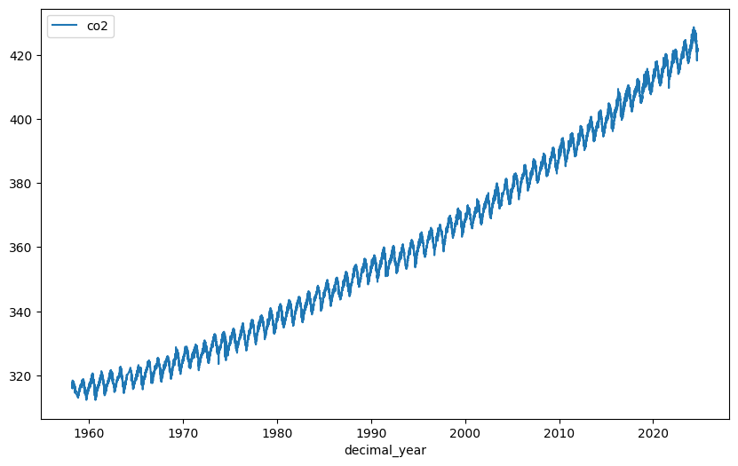
This should produce the famous ‘Keeling curve’. You will see that the carbon dioxide concentration has been increasing steadily since the earliest date in the data and also that there is a seasonal variation, i.e., the curve has a periodic fluctuation with a period of one year.

We are going to start by using a low-order polynomial to fit the basic curve and we will then introduce periodic terms to model the seasonal fluctuations. Once we have fitted the model, we will use it to try and predict the date that the CO₂ concentration will first reach 450 ppm.

Step 4 - Fitting a polynomial curve using scikit-learn

Step 4.1 - Fitting a straight line

We will start by fitting a straight line to the data using the LinearRegression class from sklearn.linear_model.

Import LinearRegression from sklearn.linear_model and make an instance of the class which you can call model. We will then use the model.fit method. The first parameter should be the decimal_year values (i.e., the x-axis values) and the second parameter should be the co2 values (i.e., the y-axis values). You can get these from the DataFrame.

An important detail: the fit method requires that the x-axis values be passed as a 2-D array, i.e., you need to ensure that the shape of the decimal_year array is (n,1) rather than (n,). You can do this using the NumPy reshape method or the expand_dims method. See the lecture notes for an example of how to do this.

After calling the fit method, you can use the model to predict CO₂ concentrations by calling the predict method and passing the decimal_year values. Store the result in a variable called co2_predicted.

Then make a plot of the original co2 values and the co2_predicted values plotted against the date. Plot these on the same axis so that you can compare the straight-line fit with the actual values.

# SOLUTION

import matplotlib
from sklearn.linear_model import LinearRegression
co2 = co2_df['co2'].array
date = co2_df['decimal_year'].array.reshape(-1,1)
model = LinearRegression()
model.fit(date, co2)
co2_predicted = model.predict(date)

plt.figure(figsize=(12, 8))
plt.plot(date, co2, label='CO2 concentration')
plt.plot(date, co2_predicted, label='CO2 concentration')

[<matplotlib.lines.Line2D at 0x7f99451034d0>]

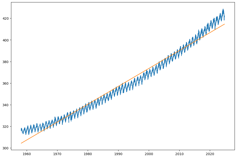
If you have done everything correctly, you should see that the straight line is a reasonable fit to the data except that it does not capture the period component and that it is too steep in the 1960s and not steep enough in the 2000s and 2010s. The pace of the CO₂ concentration increase has been increasing over time.

We can make a better fit using a higher-order polynomial with \(x^2\) and \(x^3\) terms. We will do this in the next step.

Step 4.2 - Fitting a polynomial curve

We will now fit a polynomial curve to the data. We will use the PolynomialFeatures class from sklearn.preprocessing to generate the polynomial features. We will then use the LinearRegression class to fit the model.

Import PolynomialFeatures and LinearRegression from sklearn.preprocessing and sklearn.linear_model respectively. Make an instance of the PolynomialFeatures class and call it poly. Set the degree parameter to 3. Pass the decimal_year values to the poly.fit_transform method and store the result in a variable called X. (We will use a capital X to emphasise that this is a matrix, but note that, in general, variables starting with capital letters should only be used for the names of classes).

The poly.fit_transform method returns a matrix with 4 columns. The first column is the constant term, the second column is the \(x^1\) term, the third column is the \(x^2\) term, and the fourth column is the \(x^3\) term. We will use this matrix as the input to the LinearRegression fit method.

Make an instance of the LinearRegression class and call it model. Call the model.fit method and pass the X matrix and the co2 values, just as you did in the previous step.

Now we can call model.predict and pass the X matrix again to get the predicted CO₂ concentration values. Store the result in a variable called co2_predicted.

Make a plot of the original co2 values and the co2_predicted values plotted against date. Plot these on the same axis so that you can compare the straight-line fit with the actual values.

# SOLUTION

import matplotlib
from sklearn.linear_model import LinearRegression
from sklearn.preprocessing import PolynomialFeatures

poly = PolynomialFeatures(degree=3)
co2 = co2_df['co2'].array
date = co2_df['decimal_year'].array.reshape(-1,1)
X = poly.fit_transform(date)
model = LinearRegression()
model.fit(X, co2)
co2_predicted = model.predict(X)

plt.figure(figsize=(12, 8))
plt.plot(date, co2, label='CO2 concentration')
plt.plot(date, co2_predicted, label='CO2 concentration')

[<matplotlib.lines.Line2D at 0x7f993e686c50>]

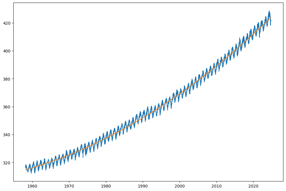
You can see that the curve fits much better to the data.

We can quantify the goodness of the fit by computing the root mean squared error (RMSE) between the predicted CO₂ values and the actual values.

We can do this easily using the root_mean_squared_error function from sklearn.metrics. Import this function and then call it passing the co2 values and the co2_predicted values.

Store the result in a variable called rmse. Print the value of rmse.

# SOLUTION

from sklearn.metrics import root_mean_squared_error

rmse = root_mean_squared_error(co2, co2_predicted)
print(f'RMSE: {rmse:.2f}')

RMSE: 2.28

Step 4.3 - Finding the best polynomial degree

In the previous section, we used a polynomial of degree 3. We did this by passing the parameter degree=3 to the PolynomialFeatures constructor. We can try different values of the degree parameter to see which gives the best fit.

In the cell below, use a loop to try values of degree from 1 to 10. For each value of degree, compute the RMSE and print it. You should be able to implement this quickly by cutting and pasting the code from the previous cells and then adding a loop around it.

# SOLUTION

from sklearn.linear_model import LinearRegression
from sklearn.preprocessing import PolynomialFeatures

co2 = co2_df['co2'].array
date = co2_df['decimal_year'].array.reshape(-1,1)

for degree in range(1, 11):
    poly = PolynomialFeatures(degree=degree)
    X = poly.fit_transform(date)
    model = LinearRegression()
    model.fit(X, co2)
    co2_predicted = model.predict(X)

    rmse = root_mean_squared_error(co2, co2_predicted)
    print(f'Degree: {degree}, RMSE: {rmse:.2f}')

Degree: 1, RMSE: 4.91
Degree: 2, RMSE: 2.28
Degree: 3, RMSE: 2.28
Degree: 4, RMSE: 2.27
Degree: 5, RMSE: 2.27
Degree: 6, RMSE: 2.27
Degree: 7, RMSE: 2.26
Degree: 8, RMSE: 2.26
Degree: 9, RMSE: 2.26
Degree: 10, RMSE: 2.26

You should find that the error drops a lot going from degree 1 to degree 2, but then only drops a little bit more going from degree 2 to degree 3. After that, the error does not drop much at all. This suggests that degree 2 or degree 3 (i.e., a 2nd or 3rd order polynomial) is the best choice.

Step 4.4 - A fairer methodology for model evaluation

In the above, we tested our model by comparing the predictions against the actual values, but we made predictions at the same dates as were used when fitting the model. This is not a fair test because the model has already seen these data points, and so it is not surprising that it fits them well. For our model to be useful, we need it to work well when predicting values for dates that it has not seen before. So to test how well we can do this, we want to fit the data using a subset of the dates (e.g., for dates up to 2000) and then test the model by predicting the values for the dates that were not used for fitting (e.g., from 2000 to 2019).

The easiest way to do this is to split our co2 and date data into two parts which we might call co2_train and date_train for the years up to 2000 and co2_test and date_test for the years from 2000 to 2019. We can then fit the model using the co2_train and date_train data and then test the model by predicting the CO₂ concentration values for the dates in date_test. We can then compare these predicted values with the actual values stored in co2_test.

We will first split the data. This can be done using the code below.

co2 = co2_df['co2'].array
date = co2_df['decimal_year'].array

date_train = date[date < 2000].reshape(-1,1)
date_test = date[date >= 2000].reshape(-1,1)
co2_train = co2[date < 2000]
co2_test = co2[date >= 2000]

Now rewrite the code from the previous section that used a loop to compute the RMSE value for polynomials of order N. But substitute date and co2 with the date_train, date_test and co2_train, co2_test values as appropriate. Note that you will also need to make separate X_train and X_test matrices using the date_train and date_test values.

# SOLUTION

import matplotlib
from sklearn.linear_model import LinearRegression
from sklearn.preprocessing import PolynomialFeatures


plt.plot(date_test, co2_test, label=f'Degree {degree}')

for degree in range(1, 11):
    poly = PolynomialFeatures(degree=degree)
    X_train = poly.fit_transform(date_train)
    X_test = poly.fit_transform(date_test)
    model = LinearRegression()
    model.fit(X_train, co2_train)
    co2_predicted = model.predict(X_test)
    plt.plot(date_test, co2_predicted, label=f'Degree {degree}')
    rmse = root_mean_squared_error(co2_test, co2_predicted)
    print(f'Degree: {degree}, RMSE: {rmse:.2f}')

Degree: 1, RMSE: 15.08
Degree: 2, RMSE: 2.66
Degree: 3, RMSE: 2.59
Degree: 4, RMSE: 2.54
Degree: 5, RMSE: 2.49
Degree: 6, RMSE: 2.45
Degree: 7, RMSE: 2.42
Degree: 8, RMSE: 2.40
Degree: 9, RMSE: 2.38
Degree: 10, RMSE: 2.37

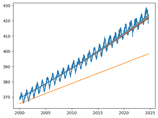
Using this more rigorous methodology, you should find that the best polynomial order is 2 rather than 3. With order 3 the predictions become quite poor. This is a case of overfitting. The model with order 3 is too complex and fits local variability in the training data that does not reflect the underlying trend.

Step 5 - Modeling the periodic component

We will now improve our model by adding periodic terms. In the lecture notes, we saw examples of how to do this by summing sine and cosine terms. For this to work, we have to assume that we know the period of the periodic component. In this case, we know that the period is one year.

Our model is going to combine the polynomial terms with the periodic terms. So, it will have the form,

\(y = a + p_1 x + p_2 x^2 + ... + p_n x^{N_\alpha} + s_1 *sin(1 \times 2 \pi x) + c_1 *cos(1 \times 2 \pi x) + ... + s_n * sin (N_\beta \times 2 \pi x) + c_n * cos (N_\beta \times 2 \pi x)\)

where \(x\) is the date in years and \(y\) is the CO₂ concentration. In the above equation, \(N_\alpha\) is the order of the polynomial and \(N_\beta\) is the number of periodic terms, and \(a\), \(p_1\), \(p_2\), …, \(p_n\), \(s_1\), \(c_1\), …, \(s_n\), \(c_n\) are the parameters that we need to estimate.

To fit this model, we will need to store the functions \(x\), \(x^2\), …, \(x^N\), and \(sin(1 \times 2 \pi x)\), \(cos(1 \times 2 \pi x)\), …, \(sin(n \times 2 \pi x)\), \(cos(n \times 2 \pi x)\) in the matrix \(X\). We will then use the LinearRegression class to fit the model in exactly the same way as we did in the previous section.

Making X with the polynomial terms is easy. We just use the PolynomialFeatures class as before. But there is no equivalent function for making the periodic terms – we need to make those using the NumPy sine and cosine functions and append them to the X matrix. See the lecture notes for an example.

Step 5.1 - Making the X matrix

In the cell below, write a function called make_features to make the X matrix for the model above. The function should take the \(x\) values (i.e., the decimal_year values) and the order of the polynomial and the number of periodic terms as parameters. Call the parameters x, order_polynomial and order_periodic respectively. It should return the \(X\) matrix.

The function can use the PolynomialFeatures class to make the polynomial terms and then append the periodic terms to the matrix. Or it may be clearer to just make both the polynomial and periodic terms using NumPy functions.

When you have written the function, run the test cell to check that it works.

# SOLUTION

def make_features(x, order_polynomial, order_periodic):

    X = np.ones((len(x), 1))
    for i in range(1, order_polynomial + 1):
        X = np.concatenate([X, x ** i], axis=1)
    for i in range(1, order_periodic + 1):
        X = np.concatenate([X, np.sin(2 * np.pi * i * x), np.cos(2 * np.pi * i * x)], axis=1)
    return X

# TEST 
x = np.linspace(0, 1, 10).reshape(-1, 1)
assert make_features(x, 2, 0).shape == (10, 3)
assert make_features(x, 0, 2).shape == (10, 5)
assert make_features(x, 2, 2).shape == (10, 7)
print('All tests passed!')

All tests passed!

Now use your function to make the feature matrix X_train for a model with polynomial order 2 and periodic order 1, i.e., by passing the model the date_train values that you used earlier.

Then make a LinearRegression model and call its fit method passing X_train and co2_train.

Finally, call model.predict with the X_train values to get the predicted CO₂ concentration values. Store the result in a variable called co2_predicted and plot the co2_predicted and co2_train values against the date_train values. You should see that the model fits the data well.

# SOLUTION

import matplotlib.pyplot as plt
from sklearn.linear_model import LinearRegression

co2 = co2_df['co2'].array
date = co2_df['decimal_year'].array.reshape(-1,1)
X_train = make_features(date_train, order_polynomial=3, order_periodic=3)
model = LinearRegression()
model.fit(X_train, co2_train)
co2_predicted = model.predict(X_train)

plt.figure(figsize=(12, 8))
plt.plot(date_train, co2_train, label='CO2 concentration')
plt.plot(date_train, co2_predicted, label='CO2 concentration')

[<matplotlib.lines.Line2D at 0x7f993e5975d0>]

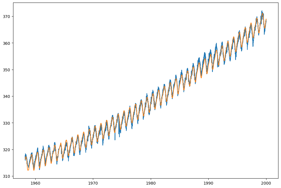
You can play with the periodic_order to see how it affects the fit. In the next section, we will try to find the best value for the periodic_order using the same methodology that we used to find the best value for the polynomial_order.

Step 5.2 - Finding the best value for the periodic order

We will now use the same methodology that we used to find the best value for the polynomial order to find the best value for the periodic order.

We will fix the polynomial order to the value of 2 but we try periodic orders from 0 to 10. In each case, we will fit the model using the date_train and co2_train values and then test the model by predicting the CO₂ concentration values for the date_test values. We will compute the RMSE value for each value of periodic order and print it to see which works best.

You should be able to do all of this using code from the previous sections.

Implement your solution in the cell below.

# SOLUTION

import matplotlib
from sklearn.linear_model import LinearRegression
from sklearn.preprocessing import PolynomialFeatures


for degree in range(0, 11):
    X_train = make_features(date_train, order_polynomial=2, order_periodic=degree)
    X_test = make_features(date_test, order_polynomial=2, order_periodic=degree)
    model = LinearRegression()
    model.fit(X_train, co2_train)
    co2_predicted = model.predict(X_test)
    rmse = root_mean_squared_error(co2_test, co2_predicted)
    print(f'Degree: {degree}, RMSE: {rmse:.2f}')

Degree: 0, RMSE: 2.66
Degree: 1, RMSE: 1.27
Degree: 2, RMSE: 1.15
Degree: 3, RMSE: 1.16
Degree: 4, RMSE: 1.16
Degree: 5, RMSE: 1.16
Degree: 6, RMSE: 1.16
Degree: 7, RMSE: 1.16

Degree: 8, RMSE: 1.16
Degree: 9, RMSE: 1.16
Degree: 10, RMSE: 1.16

You should find that the RMSE error with the periodic order set to 0 (i.e. the purely polynomial model) is about 2.57. For the periodic order set to 1 (i.e. adding in just a simple sinusoidal variation), it falls to about 1.21. Increasing to order 2 (i.e., adding a second sinusoidal term), it falls a bit further to about 1.07. After that, the prediction starts to get worse again, i.e., the model starts overfitting the data.

So, we will conclude that the best model to use is one with polynomial order 2 and periodic order 2.

Step 6 - Using our model to predict the future

We will now use our model to predict the date when the CO₂ concentration will first reach 450 ppm.

We will use the model of polynomial order 2 and periodic order 2 that we found was the best fit in the previous section. We will re-estimate the model parameters using all the data (i.e., the date and CO₂ concentration values from 1958 to 2019). We will then use the model to predict CO₂ concentration levels up to the year 2040 and look to see when this value first reaches 450 ppm.

Step 6.1 - Re-estimating the model parameters

We will first re-estimate the model parameters using all the data. This is easy to do. We just need to make the X matrix using all the dates (i.e., passing date to our make_features function). We then construct a new LinearRegression model and finally, we call the fit method on the model.

Implement this in the cell below and run the test function that will check that your model has the correct number of parameters (i.e., 7)

# SOLUTION

X = make_features(date, order_polynomial=2, order_periodic=2)
model = LinearRegression()
model.fit(X, co2)

LinearRegression()

In a Jupyter environment, please rerun this cell to show the HTML representation or trust the notebook.
On GitHub, the HTML representation is unable to render, please try loading this page with nbviewer.org.

# TEST

assert model.coef_.shape == (7,), "The model has the wrong number of coefficients"
print('All tests passed!')

All tests passed!

Step 6.2 - Predicting the future

Now, make a new date axis with dates that run all the way from 2000 to 2040.

You can do this using np.linspace to generate the date values. Choose a resolution of about 0.01 years, i.e., 100 values per year. Call this date axis date_predict.

Then pass this date axis to your make_features function to make the corresponding X matrix.

Then pass the X matrix to the model.predict method to get the predicted CO₂ concentration values. Store the result in a variable called co2_predicted.

Finally, plot the co2_predicted values against your date axis.

# SOLUTION

date_predict = np.linspace(2000, 2040, 400).reshape(-1, 1)
X_predict = make_features(date_predict, order_polynomial=2, order_periodic=2)
co2_predicted = model.predict(X_predict)
plt.plot(date_predict, co2_predicted)

[<matplotlib.lines.Line2D at 0x7f993e5643d0>]

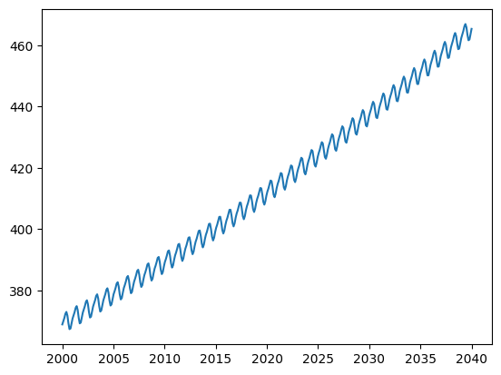
You can now find the earliest data at which the CO₂ concentration is predicted to exceed 450 ppm using something like

np.min(date_predict[co2_predicted > 450])

alternatively, you can ask for the last date at which the CO₂ concentration is predicted to fall below 450 ppm using something like

np.max(date_predict[co2_predicted < 450])

These dates are a little different due to the annual fluctuations in the CO₂ concentration.

You can compare your estimate with that made by other data scientists. There are many predictions that can be found with a bit of searching on the Web. For example, the following page has a prediction of 2037.

https://insight.factset.com/atmospheric-carbon-levels-may-2023-update#:~:text=The resulting 14.3 tells us,global warming are reached%3A 2037.

What we have to remember is that these are just predictions and that the future is uncertain. Our predictions have been made by modelling the past 60 years of data and extrapolating. This makes the big assumption that growth will continue on the same trajectory as it has in the past. Clearly, though, this is not necessarily the case. For example, as the dangers of CO₂ emissions become more apparent, governments are taking action to reduce emissions. This will (hopefully!) change the trajectory of the CO₂ concentration and so our model will no longer be valid and our predicted date will be incorrect. If emissions were cut drastically, it could even be the case that concentrations start to fall and that 450 ppm is never reached.

Conclusion

In this lab, we have used linear regression to fit a model to the atmospheric CO₂ concentration data. We have seen how to use the PolynomialFeatures class to make polynomial features and how to use the LinearRegression class to fit a model. We have also seen how to use the mean_squared_error function to compute the RMSE value for a model. We used the RMSE value to tune the hyperparameter (i.e., finding the polynomial order that produced the smallest error). We then saw how to use the np.sin and np.cos functions to make periodic features. We used these to make a model that had both polynomial and periodic terms that could fit the data much better. We then tuned the hyperparameters by training on a subset of the data and testing the model’s ability to predict the future. Finally, we used our model to predict the date when the CO₂ concentration will first reach 450 ppm.

In this lab, we have used the basic least-means-squares approach to fitting a model. This approach works well, but it can have some drawbacks. When the number of parameters is large, the model can become unstable and overfit the data. There are more sophisticated approaches that can be used to regularise the model and prevent overfitting. For example, ridge regression and lasso regression. These are implemented in the Ridge and Lasso classes in sklearn.linear_model. You can read about these in the Scikit Learn documentation.